Montefiore Medical Center/ Albert Einstein College of Medicine
What is a probabilistic sensitivity analysis?
The decision tree analysis in the base case analysis assumes that the parameters of the model are known with certainty.
In reality, the true values of these parameters are unknown. We are either estimating them from prior literature or assuming values based on expert opinion.
Instead of assigning a single fixed value to each model input (for example, “the probability of cryptococcal transmission is X%”), PSA allows each uncertain parameter to vary across a plausible range based on the available evidence. For each parameter, we specify a prior probability distribution that reflects how uncertain we are about its true value.
The cost effectiveness model is then run many times. In each run, the model randomly draws one value for each parameter from its corresponding distribution and calculates the resulting costs and health outcomes. This produces a distribution of possible results rather than a single point estimate.
For the purposes of this analysis, we have run the analysis 10,000 times.
We can plot the costs and QALYs from each simulation on a two-dimensional plot, yielding a cost-effectiveness plane. From this, we derive a 95% uncertainty ellipse1 representing the joint uncertainty of the true cost and QALY change from screening.
Source code
The probabilistic sensitivity analysis shown on this page is implemented in:
This script defines parameter distributions, runs Monte Carlo simulations, and computes expected costs and QALYs.
Parameters of the model
Probabilities
We parameterize the probability portion of the model based on the beta distribution.
The beta distribution is a way of representing uncertainty around a probability—that is, a number that must fall between 0 and 1, such as a risk, sensitivity, specificity, or event rate.
For a beta distribution with parameters \(\alpha\) and \(\beta\), the mean is given by \(\alpha / (\alpha + \beta)\). The confidence interval associated with these parameters can also be derived from these parameters.
We chose values of \(\alpha\) and \(\beta\) which yield the mean from the base case analysis and confidence intervals consistent with prior literature.
The final table is below
This yields the following parameter distributions:
Costs
We parameterize the costs portion of the model based on the gamma distribution.
The gamma distribution has a long right tail, and is therefore particularly suited for cost data, which are skewed.
For a gamma distribution with parameters \(k\) and \(\theta\), the mean is given by \(k\theta\). The confidence interval associated with these parameters can also be derived from these parameters.
We chose values of \(k\) and \(\theta\) which yield the mean from the base case analysis and confidence intervals consistent with prior literature.
Of note, since all cost data are relative to a baseline where there is no transplant performed, cost_cancellation and cost_nonacceptance are parameterized, not as functions of the gamma distribution, but as fixed constants set at 0.
The final table is below:
This yields the following parameter distributions:
QALYs
We parameterize the QALY portion of the model also based on the gamma distribution.
Again, we chose values of \(k\) and \(\theta\) which yield the mean from the base case analysis and confidence intervals consistent with prior literature.
Of note, since all QALY data are relative to a baseline where there is no transplant performed, q_noacceptance is parameterized, not as functions of the gamma distribution, but as a fixed constant set at 0.
The final table is below:
This yields the following parameter distributions:
#First, we create the dataset with the simulated values#Extract values from abovePSA_simulation<-list()PSA_simulation$probabilities <- PSA_parameters$probabilities %>%transmute(draws = purrr::map2(shape1, shape2, ~rbeta(nsim, .x, .y)) ) %>%pull(draws) %>% rlang::set_names(PSA_parameters$probabilities$parameter) %>%as_tibble()PSA_simulation$costs<-PSA_parameters$costs %>%transmute(draws = purrr::map2(shape, scale, ~rgamma(nsim, shape=.x, scale=.y)) ) %>%pull(draws) %>% rlang::set_names(PSA_parameters$costs$parameter) %>%as_tibble()%>%mutate(cost_cancellation=0,cost_nocryptococcus=-10,cost_nonacceptance=0)PSA_simulation$qalys<-PSA_parameters$qalys %>%transmute(draws = purrr::map2(shape, scale, ~rgamma(nsim, shape=.x, scale=.y)) ) %>%pull(draws) %>% rlang::set_names(PSA_parameters$qalys$parameter) %>%as_tibble()%>%mutate(q_noacceptance=0)#Combine into a single tibblePSA_simulation<-bind_cols(PSA_simulation)%>%#Add derived quantitiesmutate(p_nonusage=1-p_usage,p_donor_nocryptococcus=1-p_donor_cryptococcus,p_nontransmission=1-p_transmission,p_nospont_cryptococcus=1-p_spont_cryptococcus,p_falsenegative=1-p_sensitivity,p_falsepositive=1-p_specificity,p_nocancelled=1-p_cancelled,p_noprophrate=1-p_prophrate,p_noprophefficacy=1-p_prophefficacy,p_breakthrough_donorpos=(1-p_prophefficacy)*p_transmission,p_nobreakthrough_donorpos=1-p_breakthrough_donorpos,p_breakthrough_donorneg=(1-p_prophefficacy)*p_spont_cryptococcus,p_nobreakthrough_donorneg=1-p_breakthrough_donorneg,q_cryptococcus=q_nocryptococcus-q_loss_cryptococcus)%>%#Calculate costs and QALYsrowwise() %>%mutate(results=list(calculate_cost_QALY_QC(p_usage=p_usage, p_donor_cryptococcus=p_donor_cryptococcus, p_transmission=p_transmission,p_spont_cryptococcus=p_spont_cryptococcus,p_sensitivity=p_sensitivity,p_specificity=p_specificity,p_cancelled=p_cancelled,p_prophrate=p_prophrate,p_prophefficacy=p_prophefficacy,cost_test=cost_test,cost_disease=cost_disease,cost_fluconazole=cost_fluconazole,cost_cancellation=cost_cancellation,cost_nocryptococcus=cost_nocryptococcus,cost_nonacceptance=cost_nonacceptance,q_nocryptococcus=q_nocryptococcus,q_noacceptance=q_noacceptance,q_loss_cryptococcus=q_loss_cryptococcus )))%>%ungroup()PSA_simulation_unnested<-PSA_simulation%>%unnest(results)%>%mutate(cost_change=total_expected_cost_s-total_expected_cost_ns,qaly_change=total_expected_qaly_s-total_expected_qaly_ns)%>%mutate(icer=cost_change/qaly_change)%>%mutate(nmb = wtp * qaly_change - cost_change )#Calculate the 95% ellipsePSA_min_df <- PSA_simulation_unnested %>%select(qaly_change, cost_change)# Create mu and sigma vectors for ellipseellipse_mu <-colMeans(PSA_min_df)ellipse_Sigma <-cov(PSA_min_df)# Generate ellipse pointsellipse_df <-as.data.frame(ellipse( ellipse_Sigma,centre = ellipse_mu,level =0.95,npoints =200 ))colnames(ellipse_df) <-c("qaly_change", "cost_change")#Create PSA plotPSA_plot<-PSA_simulation_unnested%>%ggplot()+geom_point(mapping =aes(x=qaly_change, y=cost_change), alpha=0.1)+geom_path(data = ellipse_df,color ="red",mapping =aes(x=qaly_change, y=cost_change),linewidth =1 )+geom_hline(yintercept =0, linewidth =0.4, color ="black")+geom_vline(xintercept =0, linewidth =0.4, color ="black")+coord_cartesian(xlim =c(-1.5, 1.5),ylim =c(-300, 300))+theme_classic()+theme(plot.title =element_text(hjust =0.5) )+labs(title ="Probabilistic sensitivity analysis",x="QALY change",y="Cost change" )ggsave("figures/PSA_plot.svg")PSA_plot
Cost effectiveness plane
We create a cost effectiveness plane with 95% confidence ellipse marked in red below by plotting the costs from each of the simulations on the y axis and the QALYs on the x axis:
Cost-effectiveness plane showing results of the probabilistic sensitivity analysis. Each point represents one simulation; the red ellipse indicates the 95% confidence region.
Cost effectiveness acceptability curve
A cost effectiveness acceptability curve estimates the probability of screening being cost-effective as a function of the willingness-to-pay per QALY:
In this case, we see that the probability that screening is cost effective is under 10% at most reasonable thresholds of willingness-to-pay.
Summary table
We summarize our findings with the following summary table:
It is not unusual that the mean values from the PSA do not exactly correlated with the base-case results, since the outputs of the model are non-linear in their parameters.
The estimated value of perfect information (EVPI) estimates the additional financial gain per donor if all uncertainty in the parameters within the defined confidence intervals were eliminated. In this case, its low value suggests that further information would not meaningfully change the estimated NMB from screening.
This is technically a credible ellipse, since the analysis is Bayesian.↩︎
Source Code
---title: "Probabilistic sensitivity analyses"format: html---```{r setup, include=FALSE}library(here)source(here::here("R", "setup.R"))```## What is a probabilistic sensitivity analysis?The decision tree analysis in the [base case analysis](/quarto/base_case.qmd) assumes that the parameters of the model are known with certainty.In reality, the true values of these parameters are unknown. We are either estimating them from prior literature or assuming values based on expert opinion.A [**probabilistic sensitivity analysis (PSA)**](https://journals.sagepub.com/doi/10.1177/0962280211419832) is a way of explicitly ascertaining the effects of that uncertainty on a cost-effectiveness model.Instead of assigning a single fixed value to each model input (for example, “the probability of cryptococcal transmission is X%”), PSA allows each uncertain parameter to vary across a plausible range based on the available evidence. For each parameter, we specify a prior probability distribution that reflects how uncertain we are about its true value.The cost effectiveness model is then run many times. In each run, the model randomly draws one value for each parameter from its corresponding distribution and calculates the resulting costs and health outcomes. This produces a distribution of possible results rather than a single point estimate.For the purposes of this analysis, we have run the analysis `r scales::comma(nsim)` times.We can plot the costs and QALYs from each simulation on a two-dimensional plot, yielding a **cost-effectiveness plane**. From this, we derive a **95% uncertainty ellipse**[^1] representing the joint uncertainty of the true cost and QALY change from screening.[^1]: This is technically a credible ellipse, since the analysis is Bayesian.::: Rcode### Source codeThe probabilistic sensitivity analysis shown on this page is implemented in:- [`R/create_sensitivity_analysis_QC.R`](https://github.com/VagishHemmige/Cryptococcus-donor-screening-CEA/blob/master/R/create_sensitivity_analysis_QC.R)This script defines parameter distributions, runs Monte Carlo simulations, and computes expected costs and QALYs.:::## Parameters of the model### ProbabilitiesWe parameterize the probability portion of the model based on the [**beta distribution**](https://en.wikipedia.org/wiki/Beta_distribution).The beta distribution is a way of representing **uncertainty around a probability**—that is, a number that must fall between **0 and 1**, such as a risk, sensitivity, specificity, or event rate.For a beta distribution with parameters $\alpha$ and $\beta$, the mean is given by $\alpha / (\alpha + \beta)$. The confidence interval associated with these parameters can also be derived from these parameters.We chose values of $\alpha$ and $\beta$ which yield the mean from the base case analysis and confidence intervals consistent with prior literature.The final table is below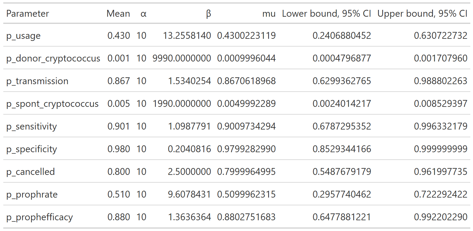This yields the following parameter distributions:::: {layout-ncol="3"}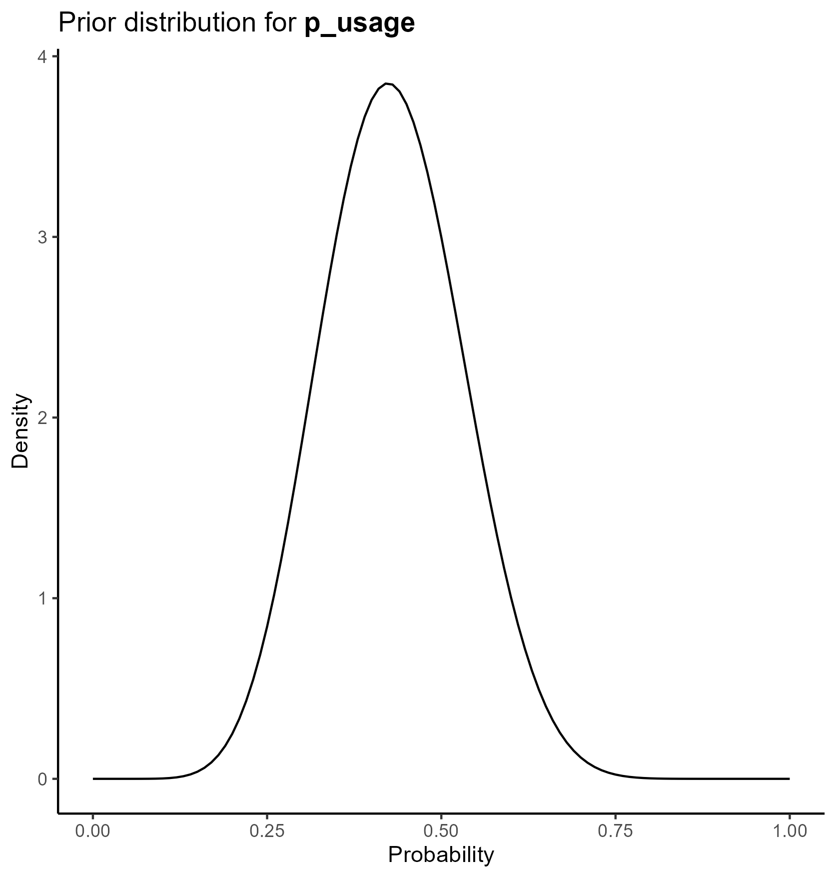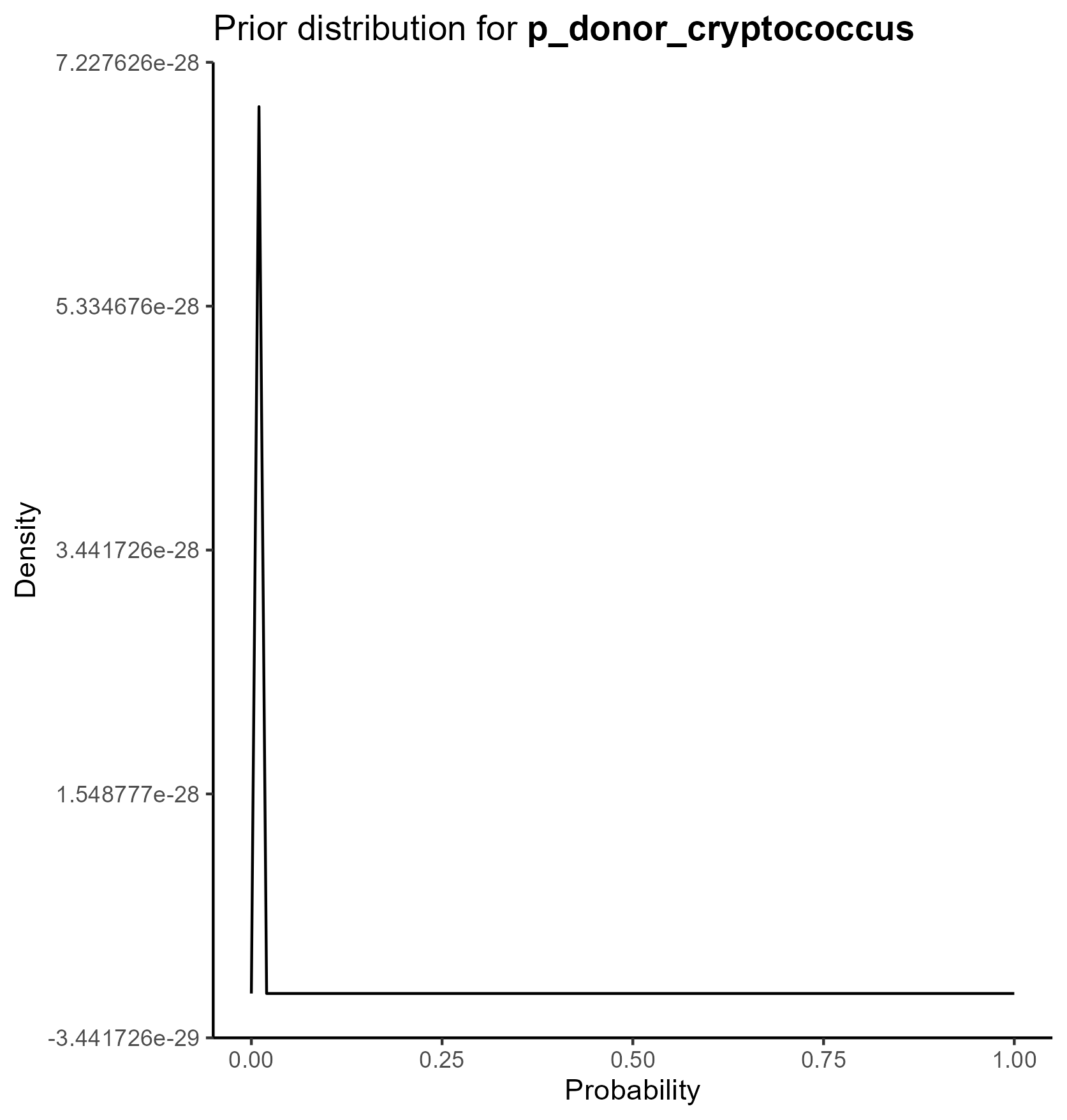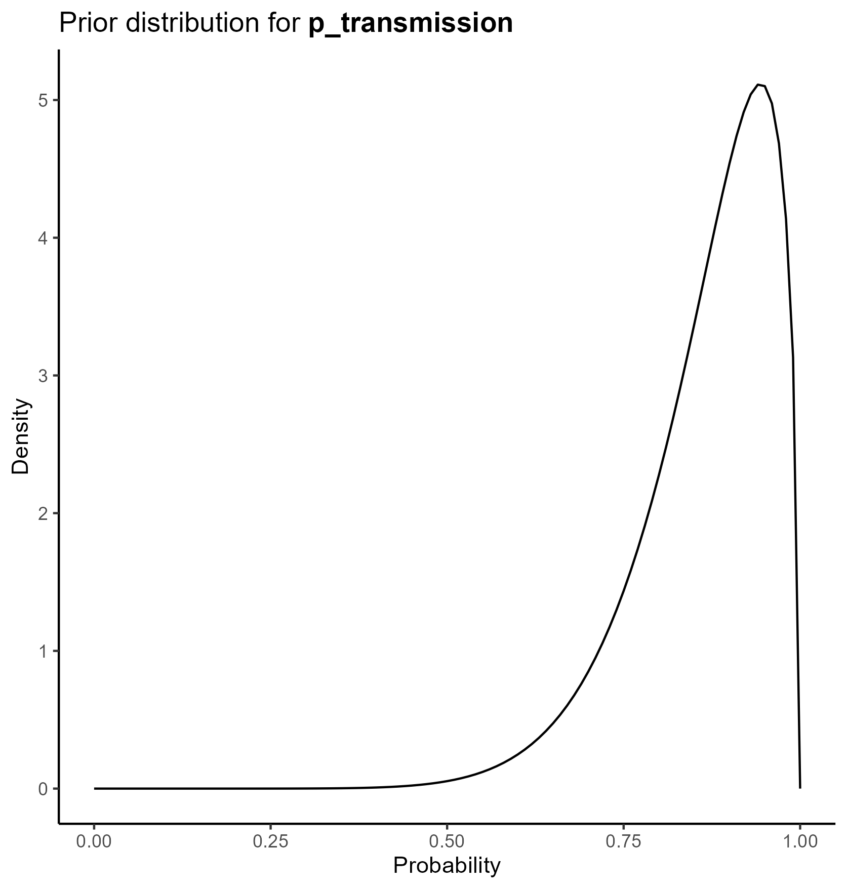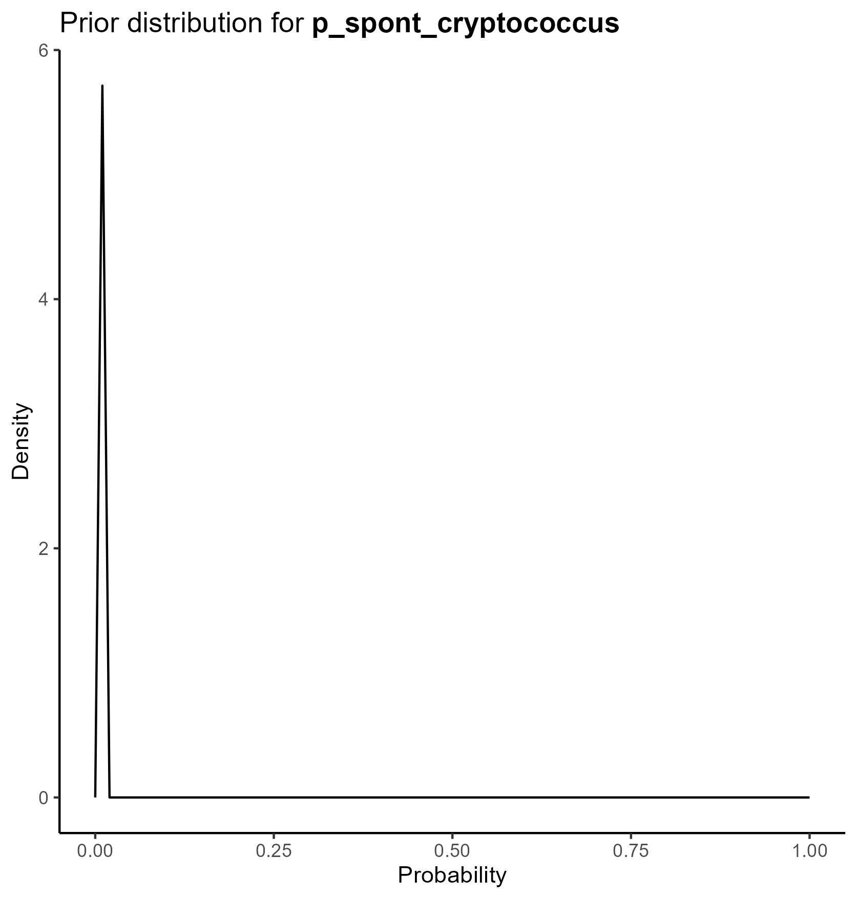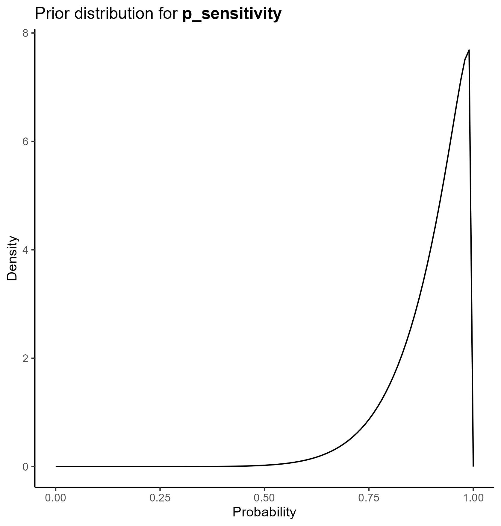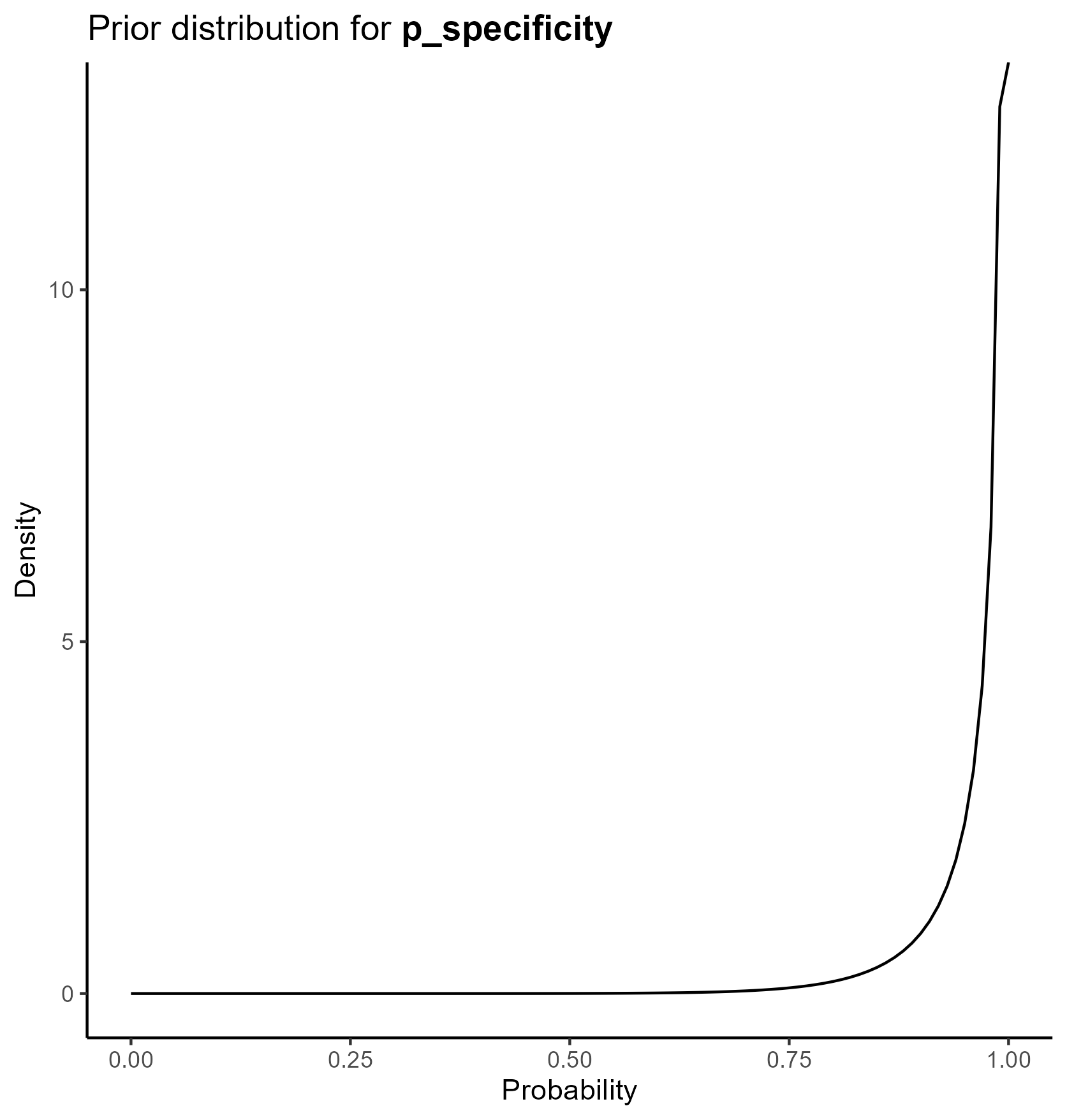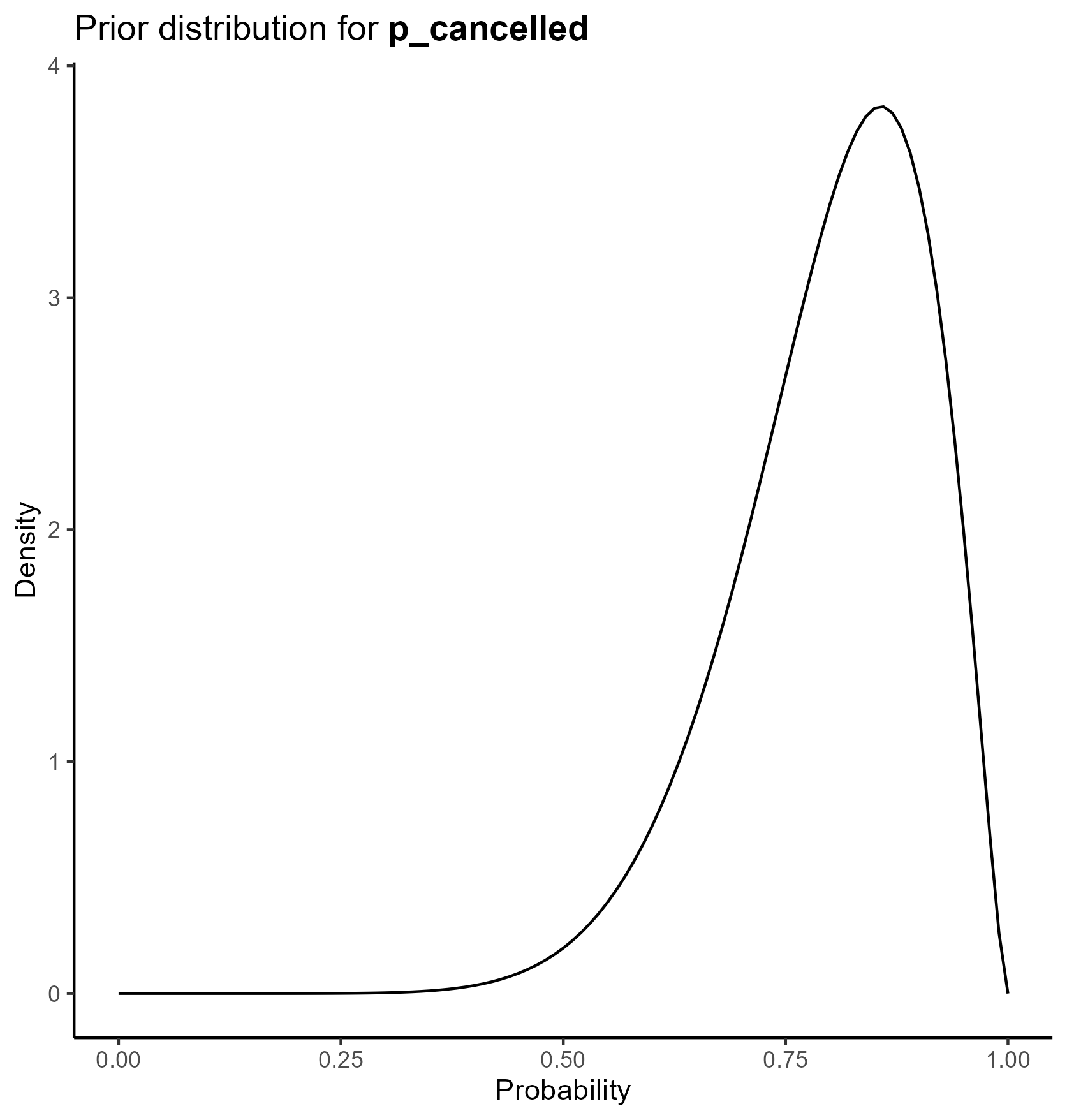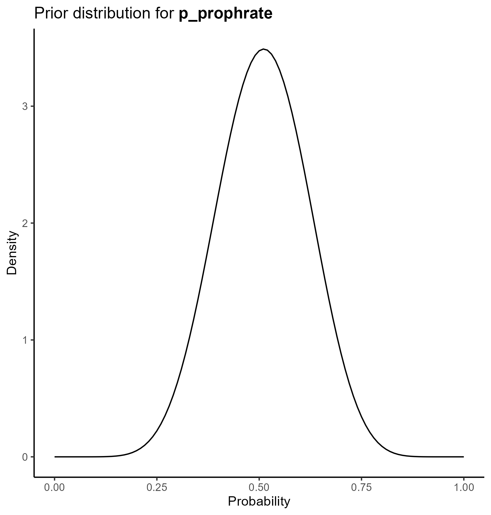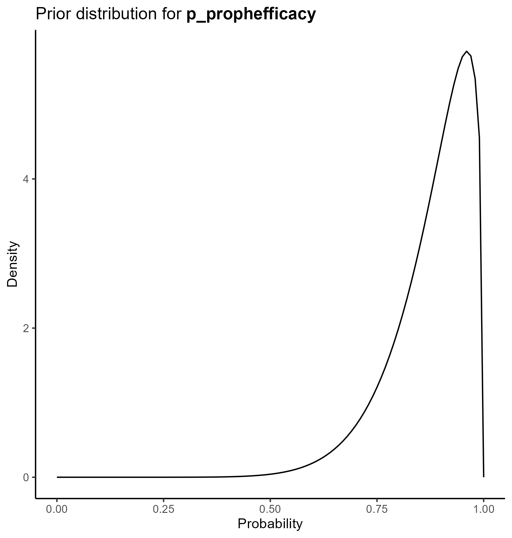:::### CostsWe parameterize the costs portion of the model based on the [**gamma distribution**](https://en.wikipedia.org/wiki/Gamma_distribution).The gamma distribution has a long right tail, and is therefore particularly suited for cost data, which are skewed.For a gamma distribution with parameters $k$ and $\theta$, the mean is given by $k\theta$. The confidence interval associated with these parameters can also be derived from these parameters.We chose values of $k$ and $\theta$ which yield the mean from the base case analysis and confidence intervals consistent with prior literature.Of note, since all cost data are relative to a baseline where there is no transplant performed, `cost_cancellation` and `cost_nonacceptance` are parameterized, not as functions of the gamma distribution, but as fixed constants set at 0.The final table is below: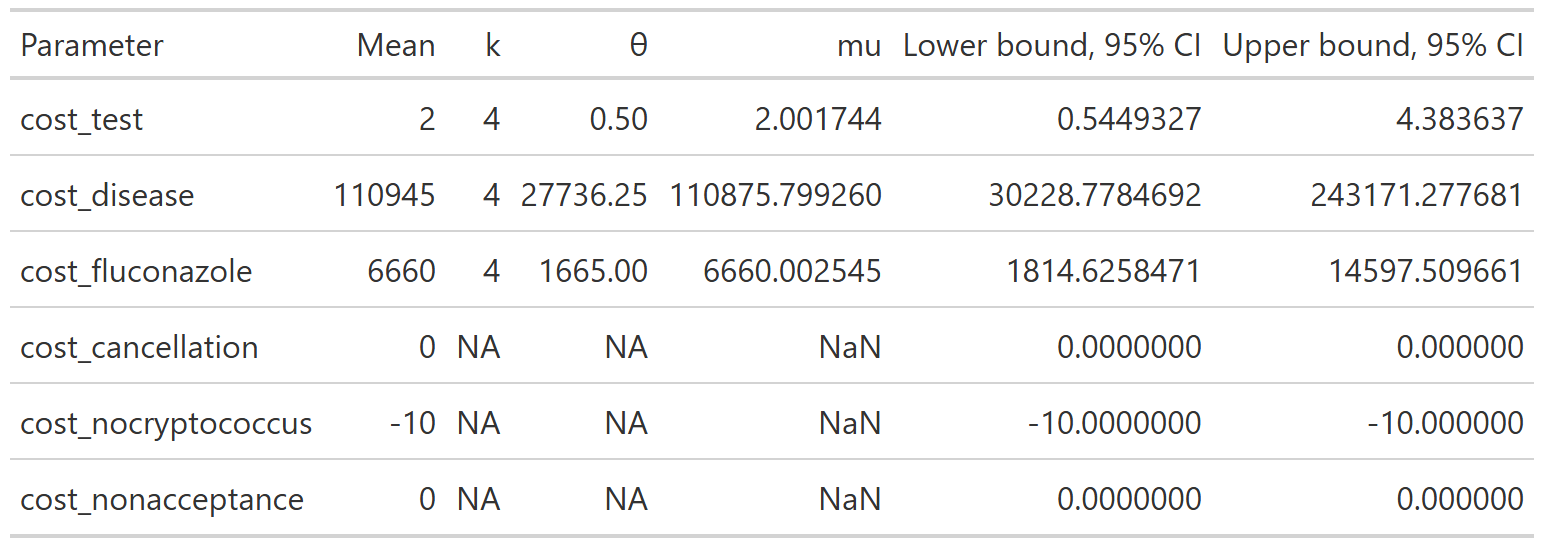This yields the following parameter distributions:::: {layout-ncol="3"}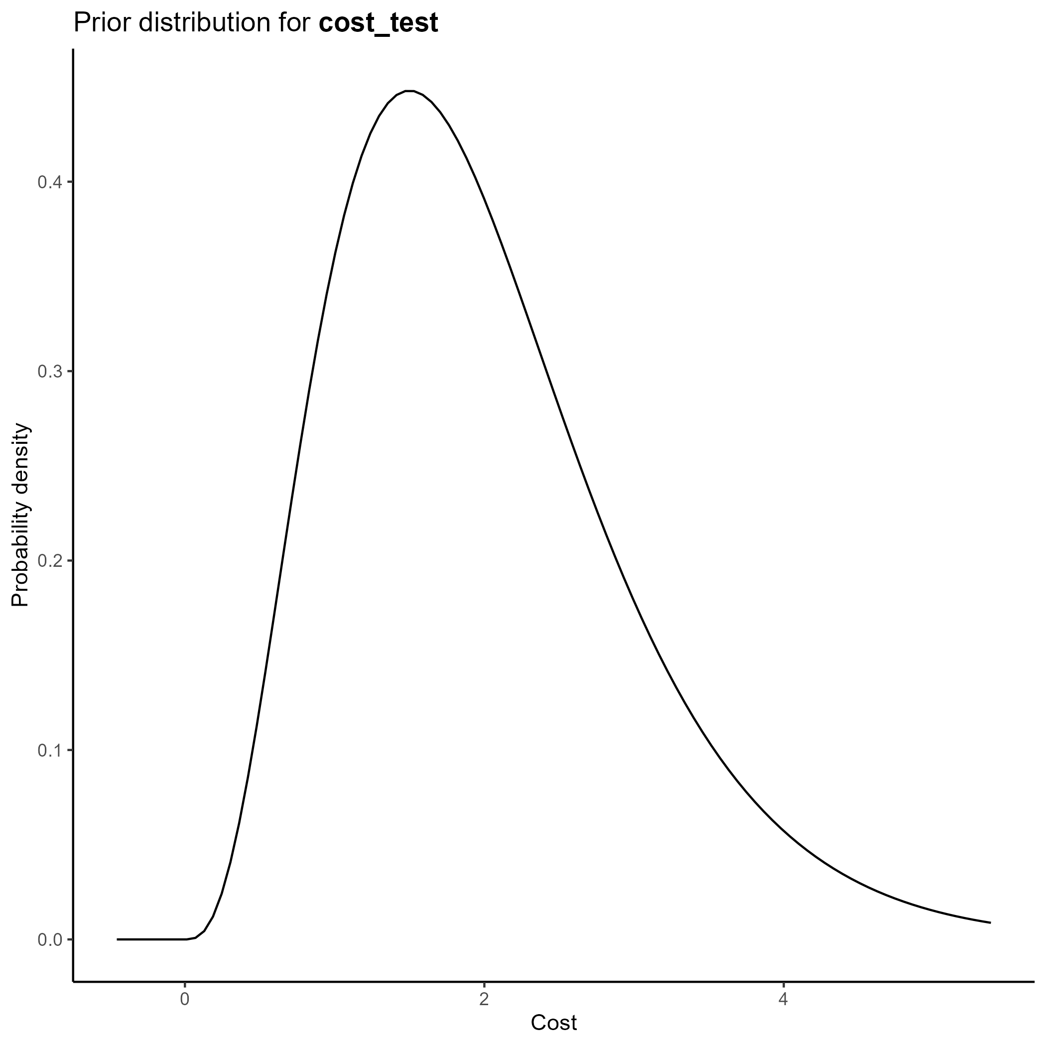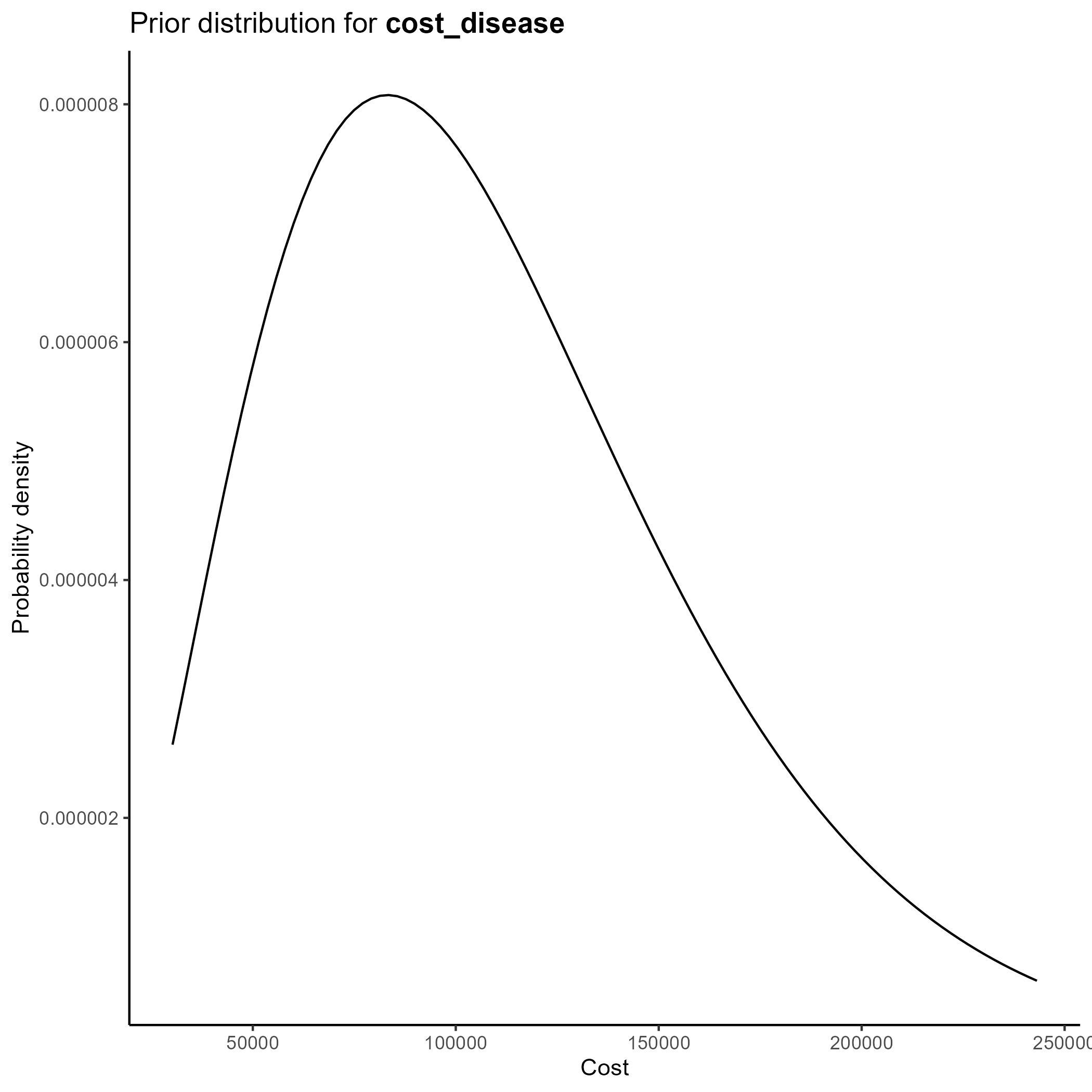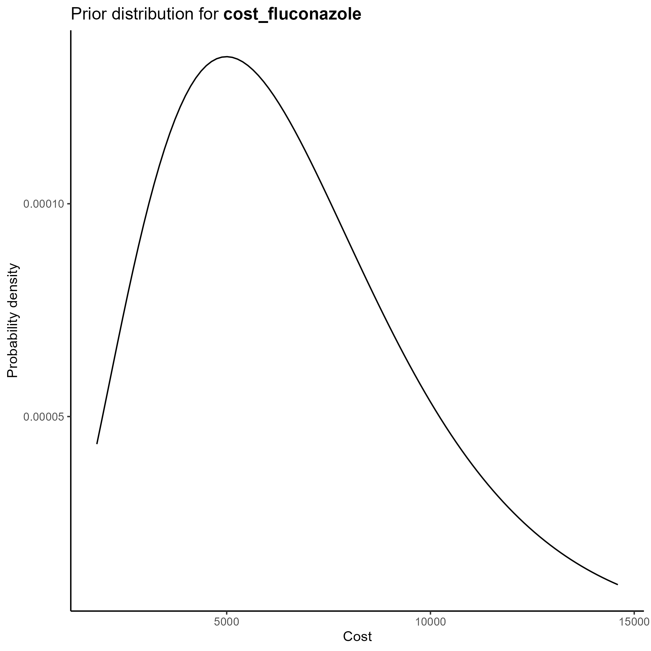:::### QALYsWe parameterize the QALY portion of the model also based on the [**gamma distribution**](https://en.wikipedia.org/wiki/Gamma_distribution).Again, we chose values of $k$ and $\theta$ which yield the mean from the base case analysis and confidence intervals consistent with prior literature.Of note, since all QALY data are relative to a baseline where there is no transplant performed, `q_noacceptance` is parameterized, not as functions of the gamma distribution, but as a fixed constant set at 0.The final table is below: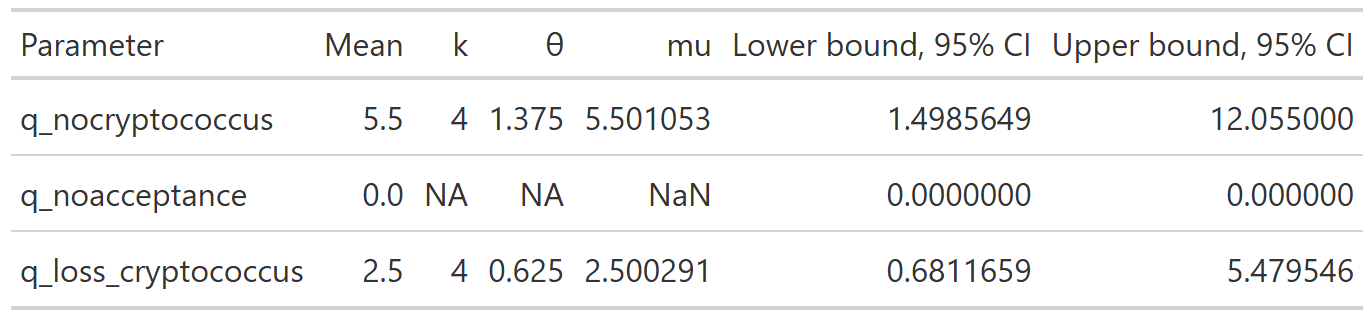This yields the following parameter distributions:::: {layout-ncol="3"}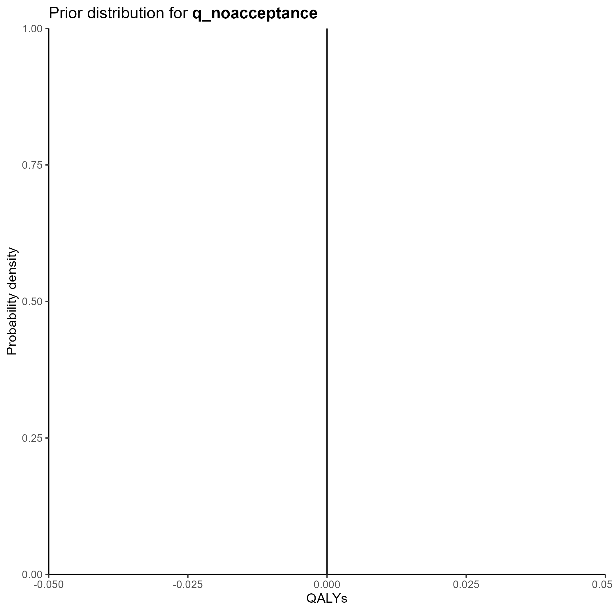:::## Source codeClick below to open up the source code from [`R/create_sensitivity_analysis_QC.R`](https://github.com/VagishHemmige/Cryptococcus-donor-screening-CEA/blob/master/R/create_sensitivity_analysis_QC.R) that is used to perform this analysis. Of note, the analysis assumes the existence of objects created in the [**One-way sensitivity analysis**](tornado.qmd) file.```{r psa_code, eval=FALSE}#First, we create the dataset with the simulated values#Extract values from abovePSA_simulation<-list()PSA_simulation$probabilities <- PSA_parameters$probabilities %>% transmute( draws = purrr::map2(shape1, shape2, ~ rbeta(nsim, .x, .y)) ) %>% pull(draws) %>% rlang::set_names(PSA_parameters$probabilities$parameter) %>% as_tibble()PSA_simulation$costs<-PSA_parameters$costs %>% transmute( draws = purrr::map2(shape, scale, ~ rgamma(nsim, shape=.x, scale=.y)) ) %>% pull(draws) %>% rlang::set_names(PSA_parameters$costs$parameter) %>% as_tibble()%>% mutate(cost_cancellation=0, cost_nocryptococcus=-10, cost_nonacceptance=0)PSA_simulation$qalys<-PSA_parameters$qalys %>% transmute( draws = purrr::map2(shape, scale, ~ rgamma(nsim, shape=.x, scale=.y)) ) %>% pull(draws) %>% rlang::set_names(PSA_parameters$qalys$parameter) %>% as_tibble()%>% mutate(q_noacceptance=0)#Combine into a single tibblePSA_simulation<-bind_cols(PSA_simulation)%>% #Add derived quantities mutate( p_nonusage=1-p_usage, p_donor_nocryptococcus=1-p_donor_cryptococcus, p_nontransmission=1-p_transmission, p_nospont_cryptococcus=1-p_spont_cryptococcus, p_falsenegative=1-p_sensitivity, p_falsepositive=1-p_specificity, p_nocancelled=1-p_cancelled, p_noprophrate=1-p_prophrate, p_noprophefficacy=1-p_prophefficacy, p_breakthrough_donorpos=(1-p_prophefficacy)*p_transmission, p_nobreakthrough_donorpos=1-p_breakthrough_donorpos, p_breakthrough_donorneg=(1-p_prophefficacy)*p_spont_cryptococcus, p_nobreakthrough_donorneg=1-p_breakthrough_donorneg, q_cryptococcus=q_nocryptococcus-q_loss_cryptococcus)%>% #Calculate costs and QALYs rowwise() %>% mutate(results=list(calculate_cost_QALY_QC(p_usage=p_usage, p_donor_cryptococcus=p_donor_cryptococcus, p_transmission=p_transmission, p_spont_cryptococcus=p_spont_cryptococcus, p_sensitivity=p_sensitivity, p_specificity=p_specificity, p_cancelled=p_cancelled, p_prophrate=p_prophrate, p_prophefficacy=p_prophefficacy, cost_test=cost_test, cost_disease=cost_disease, cost_fluconazole=cost_fluconazole, cost_cancellation=cost_cancellation, cost_nocryptococcus=cost_nocryptococcus, cost_nonacceptance=cost_nonacceptance, q_nocryptococcus=q_nocryptococcus, q_noacceptance=q_noacceptance, q_loss_cryptococcus=q_loss_cryptococcus )))%>% ungroup()PSA_simulation_unnested<-PSA_simulation%>% unnest(results)%>% mutate(cost_change=total_expected_cost_s-total_expected_cost_ns, qaly_change=total_expected_qaly_s-total_expected_qaly_ns)%>% mutate(icer=cost_change/qaly_change)%>% mutate( nmb = wtp * qaly_change - cost_change )#Calculate the 95% ellipsePSA_min_df <- PSA_simulation_unnested %>% select(qaly_change, cost_change)# Create mu and sigma vectors for ellipseellipse_mu <- colMeans(PSA_min_df)ellipse_Sigma <- cov(PSA_min_df)# Generate ellipse pointsellipse_df <- as.data.frame( ellipse( ellipse_Sigma, centre = ellipse_mu, level = 0.95, npoints = 200 ))colnames(ellipse_df) <- c("qaly_change", "cost_change")#Create PSA plotPSA_plot<-PSA_simulation_unnested%>% ggplot()+ geom_point(mapping = aes(x=qaly_change, y=cost_change), alpha=0.1)+ geom_path( data = ellipse_df, color = "red", mapping = aes(x=qaly_change, y=cost_change), linewidth = 1 )+ geom_hline(yintercept = 0, linewidth = 0.4, color = "black")+ geom_vline(xintercept = 0, linewidth = 0.4, color = "black")+ coord_cartesian(xlim = c(-1.5, 1.5), ylim = c(-300, 300))+ theme_classic()+ theme( plot.title = element_text(hjust = 0.5) )+ labs( title = "Probabilistic sensitivity analysis", x="QALY change", y="Cost change" )ggsave("figures/PSA_plot.svg")PSA_plot```## Cost effectiveness planeWe create a cost effectiveness plane with 95% confidence ellipse marked in red below by plotting the costs from each of the simulations on the y axis and the QALYs on the x axis:## Cost effectiveness acceptability curveA cost effectiveness acceptability curve estimates the probability of screening being cost-effective as a function of the willingness-to-pay per QALY:In this case, we see that the probability that screening is cost effective is under 10% at most reasonable thresholds of willingness-to-pay.## Summary tableWe summarize our findings with the following summary table:It is not unusual that the mean values from the PSA do not exactly correlated with the base-case results, since the outputs of the model are non-linear in their parameters. The [estimated value of perfect information (EVPI)](https://en.wikipedia.org/wiki/Expected_value_of_perfect_information) estimates the additional financial gain per donor if all uncertainty in the parameters within the defined confidence intervals were eliminated. In this case, its low value suggests that further information would not meaningfully change the estimated NMB from screening.## Other results- [**Base case analysis**](base_case.qmd): primary results and interpretation\- [**Additional tree analyses**](additional_trees.qmd): alternative clinical assumptions\- [**One-way sensitivity analysis**](tornado.qmd): key drivers of results\- [**About**](about.qmd): methods, assumptions, and disclosures


