Calculating geographic coverage gain
Source:vignettes/geographic-coverage-gain.Rmd
geographic-coverage-gain.RmdIntroduction
Geography matters greatly in solid organ transplantation. Donor and
recipient practices vary greatly by region, and distance-related
barriers can magnify geographic disparities. In this vignette, we
demonstrate how the calculate_geography_coverage_gain()
function can be used to estimate the number of people living with HIV
(PLWH) who gain access to heart transplant centers, defined as residence
within a 50-mile radius.
Create geography objects
We begin by using the get_hrsa_transplant_centers()
function from the sRtr package to create an sf
object containing heart transplant centers not in PR or HI. We
subsequently perform a substantial amount of data cleaning
  Transplant_centers_all_sf<-sRtr::get_hrsa_transplant_centers()%>%
    filter(OPO_STATE_ABBR != "PR" & OPO_STATE_ABBR!= "HI")%>%
    select(OTC_NM, OTC_CD, Service_Lst, X, Y) %>%
    filter(str_detect(Service_Lst, str_to_sentence("Heart")))%>%
    select(-Service_Lst)%>%
    distinct()%>%
    rename(OTCName=OTC_NM, OTCCode=OTC_CD, Latitude=Y, Longitude=X)%>%
    st_transform(5070)
We use the tigris package to import a map of states
state_geography <- tigris::states(
year = 2022,
cb = TRUE,
class = "sf")%>%
filter(!STUSPS %in% c("AK", "HI", "PR", "GU", "VI", "MP", "AS")) %>%
st_transform(5070)
#> | | | 0% | | | 1% | |= | 1% | |= | 2% | |== | 3% | |== | 4% | |=== | 4% | |=== | 5% | |==== | 5% | |==== | 6% | |===== | 7% | |===== | 8% | |====== | 8% | |====== | 9% | |======= | 10% | |======= | 11% | |======== | 11% | |======== | 12% | |========= | 13% | |========== | 14% | |========== | 15% | |=========== | 15% | |=========== | 16% | |============ | 17% | |============ | 18% | |============= | 18% | |============= | 19% | |============== | 19% | |============== | 20% | |=============== | 21% | |=============== | 22% | |================ | 22% | |================ | 23% | |================= | 24% | |================= | 25% | |================== | 25% | |================== | 26% | |=================== | 27% | |==================== | 28% | |==================== | 29% | |===================== | 29% | |===================== | 30% | |====================== | 31% | |====================== | 32% | |======================= | 32% | |======================= | 33% | |======================== | 34% | |======================== | 35% | |========================= | 35% | |========================= | 36% | |========================== | 36% | |========================== | 37% | |=========================== | 38% | |=========================== | 39% | |============================ | 40% | |============================ | 41% | |============================= | 41% | |============================= | 42% | |============================== | 42% | |============================== | 43% | |=============================== | 44% | |=============================== | 45% | |================================ | 45% | |================================ | 46% | |================================= | 47% | |================================== | 48% | |================================== | 49% | |=================================== | 50% | |=================================== | 51% | |==================================== | 51% | |==================================== | 52% | |===================================== | 53% | |====================================== | 54% | |====================================== | 55% | |======================================= | 55% | |======================================= | 56% | |======================================== | 57% | |======================================== | 58% | |========================================= | 58% | |========================================= | 59% | |========================================== | 60% | |=========================================== | 61% | |=========================================== | 62% | |============================================ | 62% | |============================================ | 63% | |============================================= | 64% | |============================================= | 65% | |============================================== | 65% | |============================================== | 66% | |=============================================== | 67% | |=============================================== | 68% | |================================================ | 68% | |================================================ | 69% | |================================================= | 69% | |================================================= | 70% | |================================================= | 71% | |================================================== | 71% | |================================================== | 72% | |=================================================== | 73% | |=================================================== | 74% | |==================================================== | 74% | |==================================================== | 75% | |===================================================== | 75% | |===================================================== | 76% | |====================================================== | 76% | |====================================================== | 77% | |======================================================= | 78% | |======================================================= | 79% | |======================================================== | 79% | |======================================================== | 80% | |======================================================== | 81% | |========================================================= | 81% | |========================================================= | 82% | |========================================================== | 82% | |========================================================== | 83% | |=========================================================== | 84% | |=========================================================== | 85% | |============================================================ | 85% | |============================================================ | 86% | |============================================================= | 87% | |============================================================= | 88% | |============================================================== | 88% | |============================================================== | 89% | |=============================================================== | 90% | |================================================================ | 91% | |================================================================ | 92% | |================================================================= | 92% | |================================================================= | 93% | |================================================================== | 94% | |================================================================== | 95% | |=================================================================== | 95% | |=================================================================== | 96% | |==================================================================== | 97% | |==================================================================== | 98% | |===================================================================== | 98% | |===================================================================== | 99% | |======================================================================| 99% | |======================================================================| 100%We use ggplot to plot the centers on a map of the United States:
ggplot()+
  geom_sf(data=state_geography)+
  geom_sf(data = Transplant_centers_all_sf)+
  theme_minimal()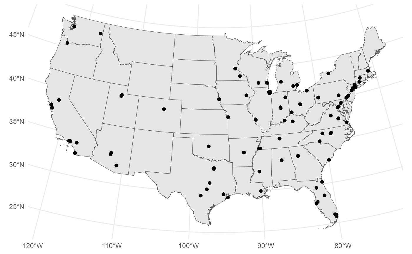
Define existing centers and additional centers
For the purposes of this analysis, we assume baseline coverage with two centers, ALUA (University of Alabama-Birmingham) and NYMA (Montefiore Medical Center).
existing_centers<-Transplant_centers_all_sf%>%
  filter(OTCCode %in% c("ALUA", "NYMA"))

ggplot()+
  geom_sf(data=state_geography)+
  geom_sf(data = existing_centers, color="red")+
  theme_minimal()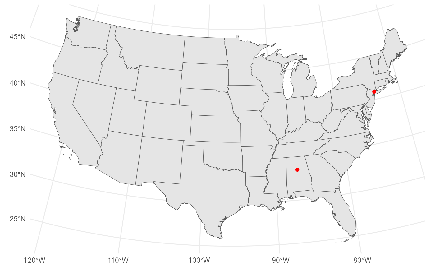
We study the additional coverage for PLWH to add NYCP (Columbia-Presbyterian) and TXHI (Texas Heart Institute at Baylor St. Luke’s Medical Center in Houston, TX).
new_centers<-Transplant_centers_all_sf%>%
  filter(OTCCode %in% c("NYCP", "TXHI"))

ggplot()+
  geom_sf(data=state_geography)+
  geom_sf(data = new_centers, color="red")+
  theme_minimal()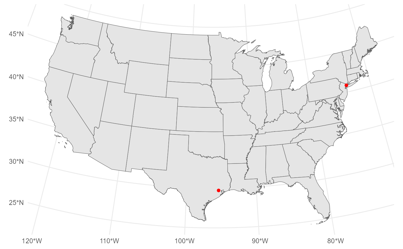
We now create 50-mile buffers (80467.2 meters) around the transplant centers in the previous objects
Transplant_centers_all_buffer<-st_buffer(Transplant_centers_all_sf,
                                        dist =80467.2)

existing_centers_buffer<-st_buffer(existing_centers,
                                   dist =80467.2)

ggplot()+
  geom_sf(data=state_geography)+
  geom_sf(data = existing_centers_buffer, color="blue")+
  geom_sf(data = existing_centers, color="red")+
  theme_minimal()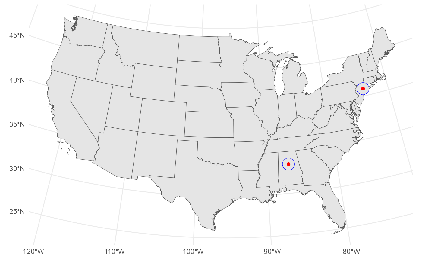
new_centers_buffer<-st_buffer(new_centers,
                              dist =80467.2)

ggplot()+
  geom_sf(data=state_geography)+
  geom_sf(data = new_centers_buffer, color="red")+
  geom_sf(data = new_centers, color="blue")+
  theme_minimal()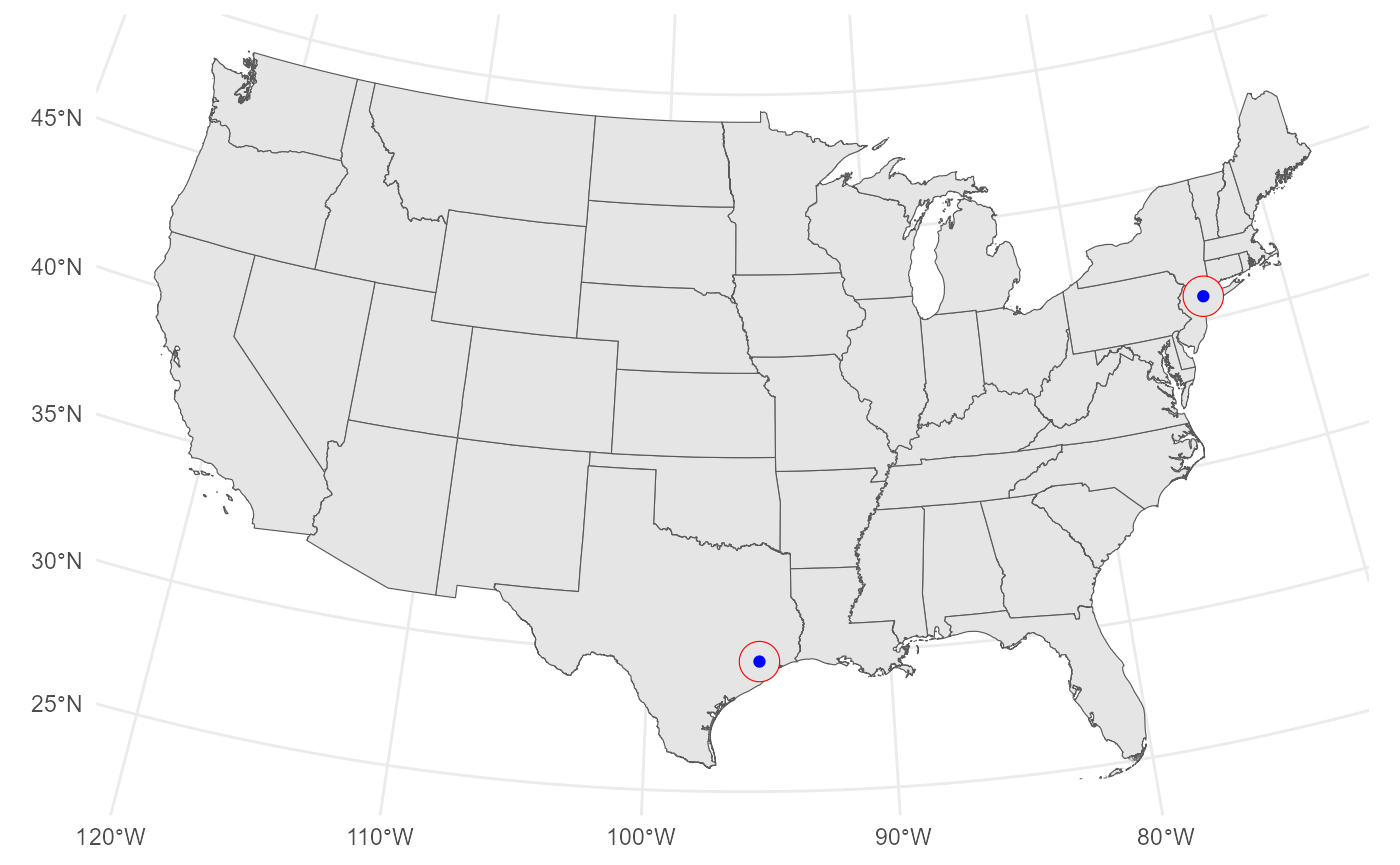
Importing HIV data
we use the CDCAtlas package to import extrapolated
estimates of the census tract-level population of PLWH, merging with
tract geography obtained via the tigris package
hiv_tract_data<-CDCAtlas::get_atlas(
disease = "hiv",
year = 2022,
geography = "county",
extrapolate_to_tract = TRUE
)%>%
filter(indicator=="HIV prevalence")
#> Joining with `by = join_by(label, concept)`
#> Getting data from the 2018-2022 5-year ACS
#> Fetching tract data by state and combining the result.
#> Joining with `by = join_by(variable)`
#> Getting data from the 2018-2022 5-year ACS
#> Joining with `by = join_by(variable)`
tract_geography <- tigris::tracts(
year = 2022,
cb = TRUE,
class = "sf"
) %>%
select(
tract_fips = GEOID,
geometry
) %>%
st_transform(5070)
#> Retrieving Census tracts for the entire United States
#> | | | 0% | | | 1% | |= | 1% | |= | 2% | |== | 2% | |== | 3% | |== | 4% | |=== | 4% | |=== | 5% | |==== | 5% | |==== | 6% | |===== | 6% | |===== | 7% | |===== | 8% | |====== | 8% | |====== | 9% | |======= | 9% | |======= | 10% | |======= | 11% | |======== | 11% | |======== | 12% | |========= | 12% | |========= | 13% | |========= | 14% | |========== | 14% | |========== | 15% | |=========== | 15% | |=========== | 16% | |============ | 16% | |============ | 17% | |============ | 18% | |============= | 18% | |============= | 19% | |============== | 19% | |============== | 20% | |============== | 21% | |=============== | 21% | |=============== | 22% | |================ | 22% | |================ | 23% | |================ | 24% | |================= | 24% | |================= | 25% | |================== | 25% | |================== | 26% | |=================== | 26% | |=================== | 27% | |=================== | 28% | |==================== | 28% | |==================== | 29% | |===================== | 29% | |===================== | 30% | |===================== | 31% | |====================== | 31% | |====================== | 32% | |======================= | 32% | |======================= | 33% | |======================= | 34% | |======================== | 34% | |======================== | 35% | |========================= | 35% | |========================= | 36% | |========================== | 36% | |========================== | 37% | |========================== | 38% | |=========================== | 38% | |=========================== | 39% | |============================ | 39% | |============================ | 40% | |============================ | 41% | |============================= | 41% | |============================= | 42% | |============================== | 42% | |============================== | 43% | |============================== | 44% | |=============================== | 44% | |=============================== | 45% | |================================ | 45% | |================================ | 46% | |================================= | 46% | |================================= | 47% | |================================= | 48% | |================================== | 48% | |================================== | 49% | |=================================== | 49% | |=================================== | 50% | |=================================== | 51% | |==================================== | 51% | |==================================== | 52% | |===================================== | 52% | |===================================== | 53% | |===================================== | 54% | |====================================== | 54% | |====================================== | 55% | |======================================= | 55% | |======================================= | 56% | |======================================== | 56% | |======================================== | 57% | |======================================== | 58% | |========================================= | 58% | |========================================= | 59% | |========================================== | 59% | |========================================== | 60% | |========================================== | 61% | |=========================================== | 61% | |=========================================== | 62% | |============================================ | 62% | |============================================ | 63% | |============================================ | 64% | |============================================= | 64% | |============================================= | 65% | |============================================== | 65% | |============================================== | 66% | |=============================================== | 66% | |=============================================== | 67% | |=============================================== | 68% | |================================================ | 68% | |================================================ | 69% | |================================================= | 69% | |================================================= | 70% | |================================================= | 71% | |================================================== | 71% | |================================================== | 72% | |=================================================== | 72% | |=================================================== | 73% | |=================================================== | 74% | |==================================================== | 74% | |==================================================== | 75% | |===================================================== | 75% | |===================================================== | 76% | |====================================================== | 76% | |====================================================== | 77% | |====================================================== | 78% | |======================================================= | 78% | |======================================================= | 79% | |======================================================== | 79% | |======================================================== | 80% | |======================================================== | 81% | |========================================================= | 81% | |========================================================= | 82% | |========================================================== | 82% | |========================================================== | 83% | |========================================================== | 84% | |=========================================================== | 84% | |=========================================================== | 85% | |============================================================ | 85% | |============================================================ | 86% | |============================================================= | 86% | |============================================================= | 87% | |============================================================= | 88% | |============================================================== | 88% | |============================================================== | 89% | |=============================================================== | 89% | |=============================================================== | 90% | |=============================================================== | 91% | |================================================================ | 91% | |================================================================ | 92% | |================================================================= | 92% | |================================================================= | 93% | |================================================================= | 94% | |================================================================== | 94% | |================================================================== | 95% | |=================================================================== | 95% | |=================================================================== | 96% | |==================================================================== | 96% | |==================================================================== | 97% | |==================================================================== | 98% | |===================================================================== | 98% | |===================================================================== | 99% | |======================================================================| 99% | |======================================================================| 100%
hiv_tract_sf <- tract_geography %>%
left_join(
hiv_tract_data,
by = "tract_fips"
)Estimating additional coverage gain
We finally use the calculate_geography_coverage_gain
function to estimate the number of PLWH who would gain geographic
proximity to a transplant center given the additional centers.
calculate_geography_coverage_gain(
    existing_areas=existing_centers_buffer,
    added_areas=new_centers_buffer,
    population_geography=hiv_tract_sf,
    coverage_vars=c("tract_cases", "tract_noncases"),
    geography_id = NULL,
    method = "intersection",
    crs = 5070,
    output = "wide"
)
#> # A tibble: 2 × 10
#>   coverage_var       total existing_covered added_covered newly_covered
#>   <chr>              <dbl>            <dbl>         <dbl>         <dbl>
#> 1 tract_cases      1099805          142598.       171835.        35318.
#> 2 tract_noncases 333270170        21744758.     27221245.      7320876.
#> # ℹ 5 more variables: combined_covered <dbl>, pct_existing_covered <dbl>,
#> #   pct_added_covered <dbl>, pct_newly_covered <dbl>,
#> #   pct_combined_covered <dbl>
We see that the additional two centers lead to an improvement in
coverage for PLWH from 142,598 PLWH to 177,917, a gain of 35,318. The
total number of PLWH in the hiv_tract_sf object is
1,099,805, consistent with the number of PLWH with known status in the
full continental US.
We also see that for people without HIV, an additional 7.3 million people gain geographical proximity with the added centers.
Starting from a NULL base
The calculate_geography_coverage_gain() function can
take a NULL input for existing_areas.
calculate_geography_coverage_gain(
    existing_areas=NULL,
    added_areas=new_centers_buffer,
    population_geography=hiv_tract_sf,
    coverage_vars=c("tract_noncases", "tract_cases"),
    geography_id = NULL,
    method = "intersection",
    crs = 5070,
    output = "wide"
)
#> # A tibble: 2 × 10
#>   coverage_var       total existing_covered added_covered newly_covered
#>   <chr>              <dbl>            <dbl>         <dbl>         <dbl>
#> 1 tract_noncases 333270170                0     27221245.     27221245.
#> 2 tract_cases      1099805                0       171835.       171835.
#> # ℹ 5 more variables: combined_covered <dbl>, pct_existing_covered <dbl>,
#> #   pct_added_covered <dbl>, pct_newly_covered <dbl>,
#> #   pct_combined_covered <dbl>
Ranking centers by incremental gain
The previous examples estimate the total population covered by a set of candidate geographic areas. In some settings, however, the goal is to compare candidate centers individually and ask which additional center would add the greatest amount of new coverage beyond an existing network.
Here, we evaluate each candidate transplant center not in the existing network one at a time. Candidate centers are defined as transplant centers that are not already included in the existing network. For each candidate center, we create a 50-mile buffer and estimate the number of additional people who would be covered if that center were added to the existing network.
Here, we create the candidate_centers_buffer object and
then pass it to the rank_individual_coverage_gains()
function, a convenient wrapper which runs the
calculate_geography_coverage_gain() function repeatedly to
generate the output table.
candidate_centers_buffer <- Transplant_centers_all_sf %>%
  filter(!(OTCCode %in% c("ALUA", "NYMA")))%>%
  st_buffer(dist = 50 * 1609.344)

ranked_gains <- rank_individual_coverage_gains(
  candidate_areas = candidate_centers_buffer,
  existing_areas = existing_centers_buffer,
  population_geography = hiv_tract_sf,
  coverage_vars = c("tract_cases", "tract_noncases"),
  method = "intersection",
  crs = 5070
)
we examine the centers with the highest additional gain and lowest additional gain.
ranked_gains$tract_cases %>%
  select(OTCName, OTCCode, newly_covered) %>%
  head(10) %>%
  gt::gt() %>%
  gt::fmt_number(
    columns = newly_covered,
    decimals = 0
  ) %>%
  gt::cols_label(
    OTCName = "Center",
    OTCCode = "Code",
    newly_covered = "Newly covered HIV prevalent cases"
)| Center | Code | Newly covered HIV prevalent cases |
|---|---|---|
| Keck Hospital of USC | CAUH | 64,983 |
| Childrens Hospital Los Angeles | CACL | 63,237 |
| Cedars-Sinai Medical Center | CACS | 61,404 |
| University of California at Los Angeles Medical Center | CAUC | 60,199 |
| Cleveland Clinic Florida Weston | FLCC | 55,824 |
| Memorial Regional Hospital/Joe DiMaggio Children's Hospital | FLJD | 55,386 |
| Memorial Regional Hospital | FLMR | 55,386 |
| Washington Hospital Center | DCWH | 52,382 |
| Children's National Medical Center | DCCH | 52,377 |
| University of Maryland Medical System | MDUM | 51,513 |
The highest yield centers are in metropolitan areas with high numbers of PLWH not served by the current network. The lowest yield are centers that are in areas with low numbers of PLWH or centers with extensive overlap with the existing centers in New York and Alabama.