
CDCAtlas provides R functions for retrieving public health surveillance data from CDC AtlasPlus.
This vignette introduces common use patterns:
- retrieving state- and county-level data
- querying different diseases
- using sex, age, and race/ethnicity stratification
- comparing rates across groups
- preparing AtlasPlus data for plotting and analysis
This vignette does not cover tract-level extrapolation. That is an advanced use case covered separately.
Installation
# install.packages("remotes")
remotes::install_github("VagishHemmige/CDCAtlas")Basic query: state-level chlamydia data
A simple query retrieves one disease, one geography level, and one year.
chlamydia_state <- get_atlas(
  disease   = "chlamydia",
  geography = "state",
  year      = 2022
)

head(chlamydia_state)
#>   indicator year  geography    data_status        race_ethnicity        sex
#> 1 Chlamydia 2022    Alabama Not Suppressed All races/ethnicities Both sexes
#> 2 Chlamydia 2022     Alaska Not Suppressed All races/ethnicities Both sexes
#> 3 Chlamydia 2022    Arizona Not Suppressed All races/ethnicities Both sexes
#> 4 Chlamydia 2022   Arkansas Not Suppressed All races/ethnicities Both sexes
#> 5 Chlamydia 2022 California Not Suppressed All races/ethnicities Both sexes
#> 6 Chlamydia 2022   Colorado Not Suppressed All races/ethnicities Both sexes
#>              age                transmission rate100000  cases population
#> 1 All age groups All transmission categories      612.1  31060    5074296
#> 2 All age groups All transmission categories      727.7   5338     733583
#> 3 All age groups All transmission categories      554.4  40796    7359197
#> 4 All age groups All transmission categories      588.3  17918    3045637
#> 5 All age groups All transmission categories      493.6 192647   39029342
#> 6 All age groups All transmission categories      456.3  26646    5839926
#>   lowerci_rate upperci_rate rse lowerci_cases upperci_cases fips
#> 1           NA           NA  NA            NA            NA   01
#> 2           NA           NA  NA            NA            NA   02
#> 3           NA           NA  NA            NA            NA   04
#> 4           NA           NA  NA            NA            NA   05
#> 5           NA           NA  NA            NA            NA   06
#> 6           NA           NA  NA            NA            NA   08
The returned object is a data frame that can be used directly with tidyverse tools.
glimpse(chlamydia_state)
#> Rows: 57
#> Columns: 17
#> $ indicator      <fct> "Chlamydia", "Chlamydia", "Chlamydia", "Chlamydia", "Ch…
#> $ year           <dbl> 2022, 2022, 2022, 2022, 2022, 2022, 2022, 2022, 2022, 2…
#> $ geography      <fct> "Alabama", "Alaska", "Arizona", "Arkansas", "California…
#> $ data_status    <fct> "Not Suppressed", "Not Suppressed", "Not Suppressed", "…
#> $ race_ethnicity <fct> "All races/ethnicities", "All races/ethnicities", "All …
#> $ sex            <fct> "Both sexes", "Both sexes", "Both sexes", "Both sexes",…
#> $ age            <fct> "All age groups", "All age groups", "All age groups", "…
#> $ transmission   <fct> "All transmission categories", "All transmission catego…
#> $ rate100000     <dbl> 612.1, 727.7, 554.4, 588.3, 493.6, 456.3, 143.8, 593.9,…
#> $ cases          <dbl> 31060, 5338, 40796, 17918, 192647, 26646, 4633, 626, NA…
#> $ population     <dbl> 5074296, 733583, 7359197, 3045637, 39029342, 5839926, 3…
#> $ lowerci_rate   <dbl> NA, NA, NA, NA, NA, NA, NA, NA, NA, NA, NA, NA, NA, NA,…
#> $ upperci_rate   <dbl> NA, NA, NA, NA, NA, NA, NA, NA, NA, NA, NA, NA, NA, NA,…
#> $ rse            <dbl> NA, NA, NA, NA, NA, NA, NA, NA, NA, NA, NA, NA, NA, NA,…
#> $ lowerci_cases  <dbl> NA, NA, NA, NA, NA, NA, NA, NA, NA, NA, NA, NA, NA, NA,…
#> $ upperci_cases  <dbl> NA, NA, NA, NA, NA, NA, NA, NA, NA, NA, NA, NA, NA, NA,…
#> $ fips           <chr> "01", "02", "04", "05", "06", "08", "72", "78", "70", "…
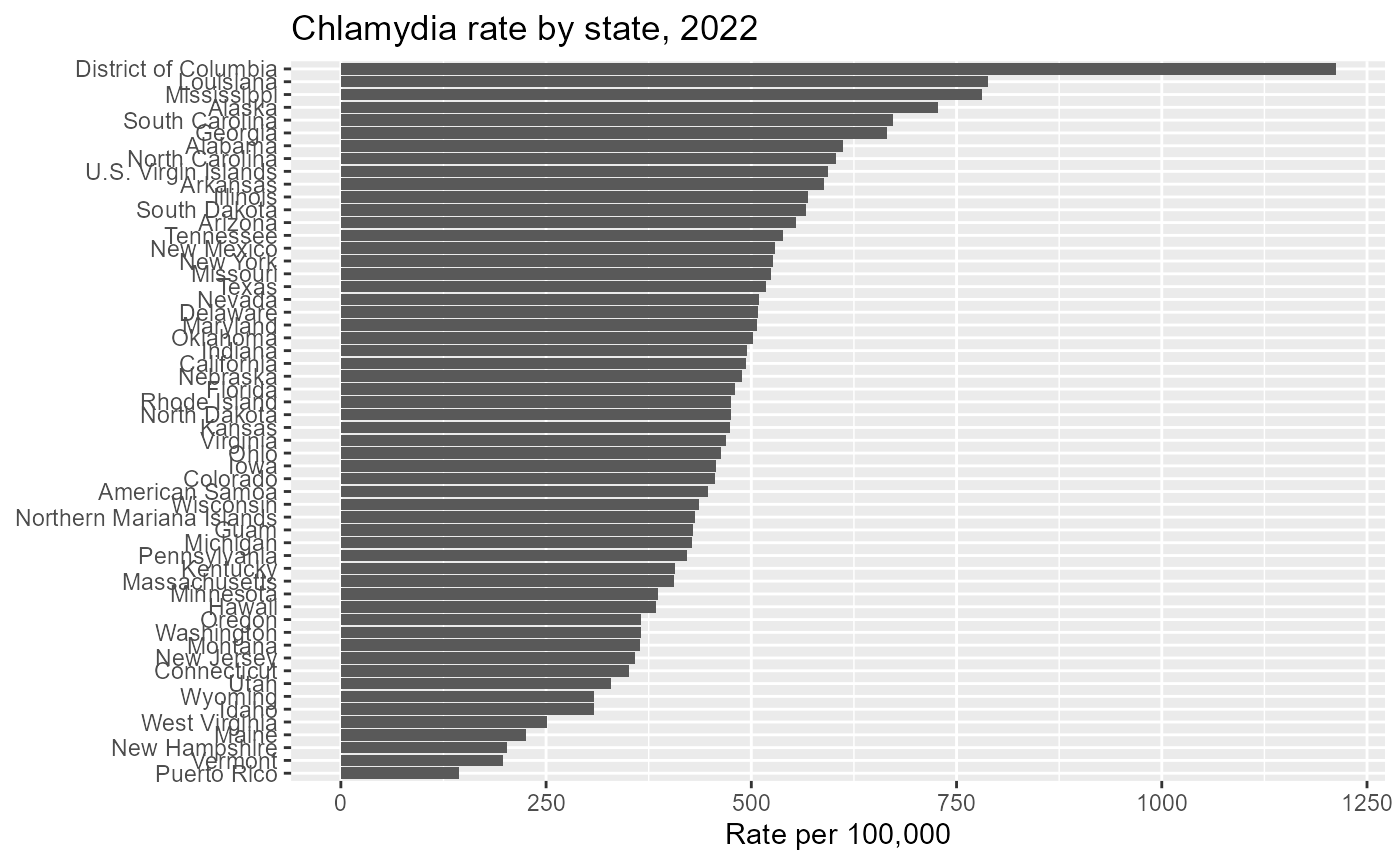
Plot state-level rates
chlamydia_state %>%
  filter(!is.na(rate100000)) %>%
  ggplot(aes(x = reorder(geography, rate100000), y = rate100000)) +
  geom_col() +
  coord_flip() +
  labs(
    title = "Chlamydia rate by state, 2022",
    x = NULL,
    y = "Rate per 100,000"
  )
Query county-level data
AtlasPlus can also return county-level data for supported diseases.
chlamydia_county <- get_atlas(
  disease   = "chlamydia",
  geography = "county",
  year      = 2022
)

head(chlamydia_county)
#>   indicator year            geography    data_status        race_ethnicity
#> 1 Chlamydia 2022 Abbeville County, SC Not Suppressed All races/ethnicities
#> 2 Chlamydia 2022       Ada County, ID Not Suppressed All races/ethnicities
#> 3 Chlamydia 2022     Adair County, IA Not Suppressed All races/ethnicities
#> 4 Chlamydia 2022    Acadia Parish, LA Not Suppressed All races/ethnicities
#> 5 Chlamydia 2022  Accomack County, VA Not Suppressed All races/ethnicities
#> 6 Chlamydia 2022     Adams County, CO Not Suppressed All races/ethnicities
#>          sex            age                transmission rate100000 cases
#> 1 Both sexes All age groups All transmission categories      496.8   121
#> 2 Both sexes All age groups All transmission categories      403.3  2093
#> 3 Both sexes All age groups All transmission categories      186.8    14
#> 4 Both sexes All age groups All transmission categories      676.7   384
#> 5 Both sexes All age groups All transmission categories      524.2   174
#> 6 Both sexes All age groups All transmission categories      591.8  3122
#>   population lowerci_rate upperci_rate rse lowerci_cases upperci_cases  fips
#> 1      24356           NA           NA  NA            NA            NA 45001
#> 2     518907           NA           NA  NA            NA            NA 16001
#> 3       7494           NA           NA  NA            NA            NA 19001
#> 4      56744           NA           NA  NA            NA            NA 22001
#> 5      33191           NA           NA  NA            NA            NA 51001
#> 6     527575           NA           NA  NA            NA            NA 08001
A common workflow is to identify counties with the highest reported rates.
chlamydia_county %>%
  filter(!is.na(rate100000)) %>%
  arrange(desc(rate100000)) %>%
  select(geography, cases, rate100000) %>%
  head(10)
#>                       geography cases rate100000
#> 1             Reeves County, TX   552     4277.4
#> 2               Todd County, SD   340     3687.6
#> 3      Kusilvak Census Area, AK   287     3467.0
#> 4              Dewey County, SD   174     3385.2
#> 5        Bethel Census Area, AK   528     2892.0
#> 6          Nome Census Area, AK   281     2857.1
#> 7      Oglala Lakota County, SD   359     2655.5
#> 8           Mellette County, SD    40     2114.2
#> 9  Northwest Arctic Borough, AK   150     2020.7
#> 10            Tunica County, MS   186     1966.6
Stratification by sex
Many AtlasPlus endpoints support stratification. For example, we can retrieve state-level gonorrhea data by sex.
gonorrhea_sex <- get_atlas(
  disease   = "gonorrhea",
  geography = "state",
  year      = 2022,
  stratify_by = "sex"
)

head(gonorrhea_sex)
#>   indicator year geography    data_status        race_ethnicity    sex
#> 1 Gonorrhea 2022   Alabama Not Suppressed All races/ethnicities   Male
#> 2 Gonorrhea 2022   Alabama Not Suppressed All races/ethnicities Female
#> 3 Gonorrhea 2022    Alaska Not Suppressed All races/ethnicities   Male
#> 4 Gonorrhea 2022    Alaska Not Suppressed All races/ethnicities Female
#> 5 Gonorrhea 2022   Arizona Not Suppressed All races/ethnicities   Male
#> 6 Gonorrhea 2022   Arizona Not Suppressed All races/ethnicities Female
#>              age                transmission rate100000 cases population
#> 1 All age groups All transmission categories      279.7  6901    2467360
#> 2 All age groups All transmission categories      238.3  6213    2606936
#> 3 All age groups All transmission categories      296.7  1145     385947
#> 4 All age groups All transmission categories      333.4  1159     347636
#> 5 All age groups All transmission categories      270.1  9936    3679034
#> 6 All age groups All transmission categories      177.2  6522    3680163
#>   lowerci_rate upperci_rate rse lowerci_cases upperci_cases fips
#> 1           NA           NA  NA            NA            NA   01
#> 2           NA           NA  NA            NA            NA   01
#> 3           NA           NA  NA            NA            NA   02
#> 4           NA           NA  NA            NA            NA   02
#> 5           NA           NA  NA            NA            NA   04
#> 6           NA           NA  NA            NA            NA   04
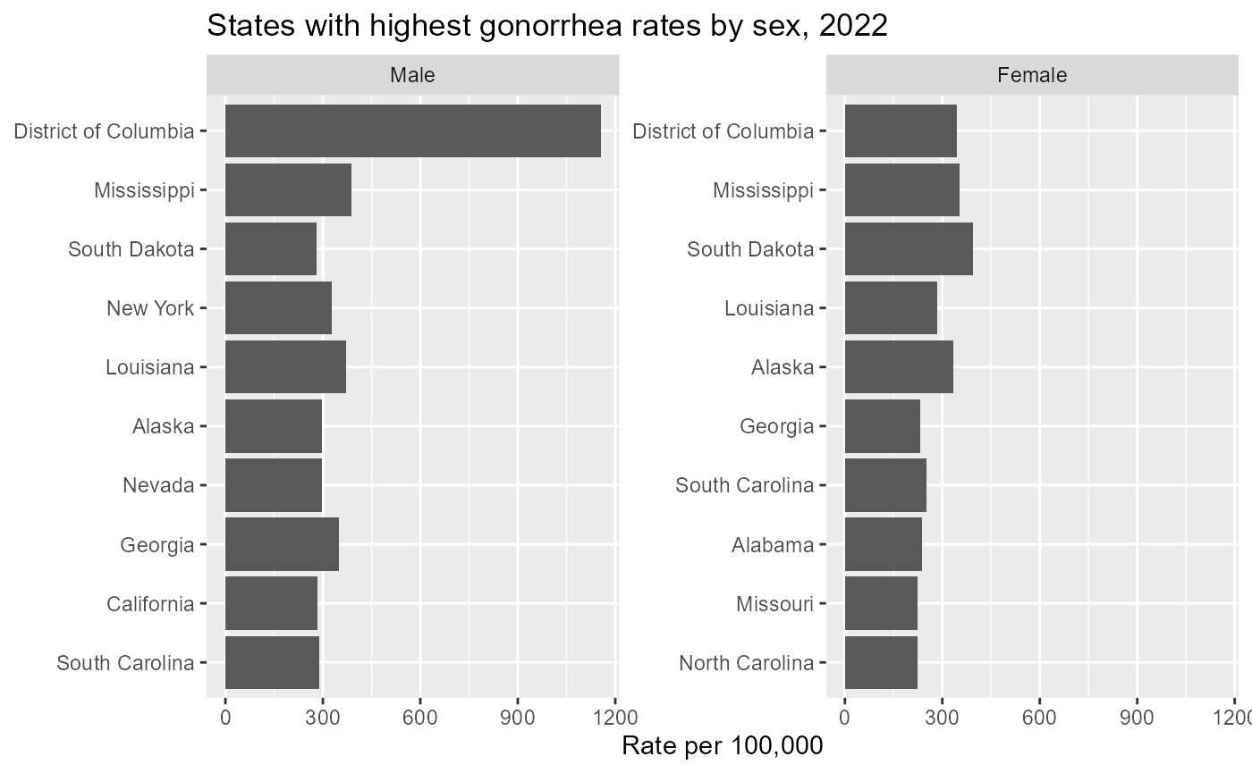
Now we can compare rates by sex within each state.
gonorrhea_sex %>%
  filter(!is.na(rate100000)) %>%
  group_by(sex) %>%
  slice_max(rate100000, n = 10, with_ties = FALSE) %>%
  ungroup() %>%
  ggplot(aes(x = reorder(geography, rate100000), y = rate100000)) +
  geom_col() +
  coord_flip() +
  facet_wrap(~ sex, scales = "free_y") +
  labs(
    title = "States with highest gonorrhea rates by sex, 2022",
    x = NULL,
    y = "Rate per 100,000"
  )
Stratification by age
AtlasPlus also supports age-stratified queries for many disease/geography combinations.
hiv_age <- get_atlas(
  disease   = "hiv",
  geography = "state",
  year      = 2022,
  stratify_by = "age"

)

head(hiv_age)
#>       indicator year geography    data_status        race_ethnicity        sex
#> 1 HIV diagnoses 2022   Alabama Not Suppressed All races/ethnicities Both sexes
#> 2 HIV diagnoses 2022   Alabama Not Suppressed All races/ethnicities Both sexes
#> 3 HIV diagnoses 2022   Alabama Not Suppressed All races/ethnicities Both sexes
#> 4 HIV diagnoses 2022   Alabama Not Suppressed All races/ethnicities Both sexes
#> 5 HIV diagnoses 2022   Alabama Not Suppressed All races/ethnicities Both sexes
#> 6 HIV diagnoses 2022   Alabama Not Suppressed All races/ethnicities Both sexes
#>     age                transmission rate100000 cases population lowerci_rate
#> 1 13-24 All transmission categories       19.9   162     812982           NA
#> 2 25-34 All transmission categories       34.5   227     657946           NA
#> 3 35-44 All transmission categories       24.0   150     625076           NA
#> 4 45-54 All transmission categories       13.6    84     618962           NA
#> 5 55-64 All transmission categories        8.2    54     660461           NA
#> 6   65+ All transmission categories        1.3    12     905888           NA
#>   upperci_rate rse lowerci_cases upperci_cases fips
#> 1           NA  NA            NA            NA   01
#> 2           NA  NA            NA            NA   01
#> 3           NA  NA            NA            NA   01
#> 4           NA  NA            NA            NA   01
#> 5           NA  NA            NA            NA   01
#> 6           NA  NA            NA            NA   01
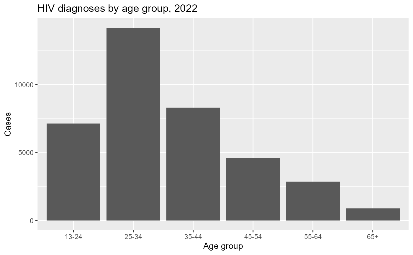
We can summarize national patterns by aggregating across states.
hiv_age_summary <- hiv_age %>%
  group_by(age, indicator) %>%
  summarize(
    cases = sum(cases, na.rm = TRUE),
    .groups = "drop"
  )

hiv_age_summary
#> # A tibble: 12 × 3
#>    age   indicator       cases
#>    <fct> <fct>           <dbl>
#>  1 13-24 HIV diagnoses    7142
#>  2 13-24 HIV prevalence  28242
#>  3 25-34 HIV diagnoses   14195
#>  4 25-34 HIV prevalence 166643
#>  5 35-44 HIV diagnoses    8320
#>  6 35-44 HIV prevalence 212167
#>  7 45-54 HIV diagnoses    4601
#>  8 45-54 HIV prevalence 238245
#>  9 55-64 HIV diagnoses    2873
#> 10 55-64 HIV prevalence 296458
#> 11 65+   HIV diagnoses     887
#> 12 65+   HIV prevalence 162449
hiv_age_summary%>%
  filter(indicator=="HIV diagnoses")%>%
  ggplot(mapping=aes(x = age, y = cases)) +
  geom_col() +
  labs(
    title = "HIV diagnoses by age group, 2022",
    x = "Age group",
    y = "Cases"
  )
Stratification by race/ethnicity
CDC AtlasPlus commonly uses a combined race/ethnicity variable rather than separate race and Hispanic ethnicity fields.
hiv_race <- get_atlas(
  disease        = "hiv",
  geography      = "state",
  year           = 2022,
  stratify_by = "race"

)

head(hiv_race)
#>       indicator year geography    data_status
#> 1 HIV diagnoses 2022   Alabama Not Suppressed
#> 2 HIV diagnoses 2022   Alabama Not Suppressed
#> 3 HIV diagnoses 2022   Alabama Not Suppressed
#> 4 HIV diagnoses 2022   Alabama Not Suppressed
#> 5 HIV diagnoses 2022   Alabama Not Suppressed
#> 6 HIV diagnoses 2022   Alabama Not Suppressed
#>                           race_ethnicity        sex                     age
#> 1          American Indian/Alaska Native Both sexes Ages 13 years and older
#> 2                                  Asian Both sexes Ages 13 years and older
#> 3                 Black/African American Both sexes Ages 13 years and older
#> 4                        Hispanic/Latino Both sexes Ages 13 years and older
#> 5 Native Hawaiian/Other Pacific Islander Both sexes Ages 13 years and older
#> 6                                  White Both sexes Ages 13 years and older
#>                  transmission rate100000 cases population lowerci_rate
#> 1 All transmission categories        7.9     2      25389           NA
#> 2 All transmission categories        3.0     2      66122           NA
#> 3 All transmission categories       39.1   434    1109054           NA
#> 4 All transmission categories       20.8    42     202304           NA
#> 5 All transmission categories       45.8     1       2184           NA
#> 6 All transmission categories        5.9   167    2819309           NA
#>   upperci_rate rse lowerci_cases upperci_cases fips
#> 1           NA  NA            NA            NA   01
#> 2           NA  NA            NA            NA   01
#> 3           NA  NA            NA            NA   01
#> 4           NA  NA            NA            NA   01
#> 5           NA  NA            NA            NA   01
#> 6           NA  NA            NA            NA   01
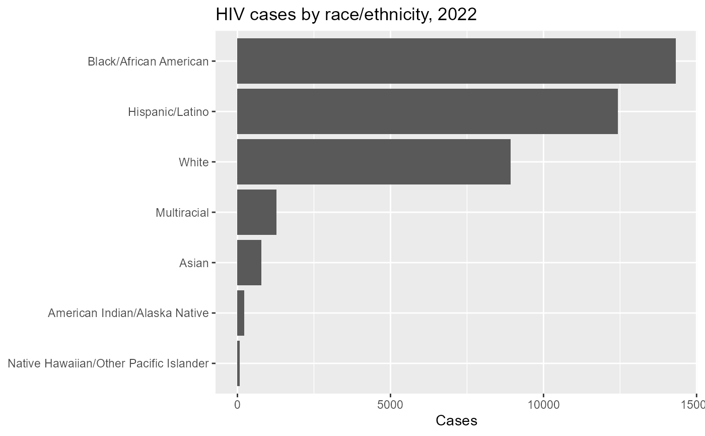
A useful first look is to compare total reported cases by race/ethnicity.
hiv_race_summary <- hiv_race %>%
  group_by(race_ethnicity, indicator) %>%
  summarize(
    cases = sum(cases, na.rm = TRUE),
    .groups = "drop"
  ) %>%
  arrange(desc(cases))

hiv_race_summary
#> # A tibble: 14 × 3
#>    race_ethnicity                         indicator       cases
#>    <fct>                                  <fct>           <dbl>
#>  1 Black/African American                 HIV prevalence 429419
#>  2 White                                  HIV prevalence 303461
#>  3 Hispanic/Latino                        HIV prevalence 287681
#>  4 Multiracial                            HIV prevalence  61928
#>  5 Asian                                  HIV prevalence  17020
#>  6 Black/African American                 HIV diagnoses   14319
#>  7 Hispanic/Latino                        HIV diagnoses   12422
#>  8 White                                  HIV diagnoses    8923
#>  9 American Indian/Alaska Native          HIV prevalence   3148
#> 10 Multiracial                            HIV diagnoses    1276
#> 11 Native Hawaiian/Other Pacific Islander HIV prevalence    919
#> 12 Asian                                  HIV diagnoses     784
#> 13 American Indian/Alaska Native          HIV diagnoses     216
#> 14 Native Hawaiian/Other Pacific Islander HIV diagnoses      78
hiv_race_summary%>%
  filter(indicator=="HIV diagnoses")%>%
  ggplot(mapping =aes(x = reorder(race_ethnicity, cases), y = cases)) +
  geom_col() +
  coord_flip() +
  labs(
    title = "HIV cases by race/ethnicity, 2022",
    x = NULL,
    y = "Cases"
  )
Multiple stratification variables
You can request combinations of stratification variables when supported by the underlying AtlasPlus endpoint. For example, HIV data can be queried by both sex and age.
hiv_age_sex <- get_atlas(
  disease   = "hiv",
  geography = "state",
  year      = 2022,
  stratify_by = c("sex", "age")

)

head(hiv_age_sex)
#>       indicator year geography    data_status        race_ethnicity  sex   age
#> 1 HIV diagnoses 2022   Alabama Not Suppressed All races/ethnicities Male 13-24
#> 2 HIV diagnoses 2022   Alabama Not Suppressed All races/ethnicities Male 25-34
#> 3 HIV diagnoses 2022   Alabama Not Suppressed All races/ethnicities Male 35-44
#> 4 HIV diagnoses 2022   Alabama Not Suppressed All races/ethnicities Male 45-54
#> 5 HIV diagnoses 2022   Alabama Not Suppressed All races/ethnicities Male 55-64
#> 6 HIV diagnoses 2022   Alabama Not Suppressed All races/ethnicities Male   65+
#>                  transmission rate100000 cases population lowerci_rate
#> 1 All transmission categories       34.9   143     410156           NA
#> 2 All transmission categories       57.8   188     325041           NA
#> 3 All transmission categories       33.6   102     303880           NA
#> 4 All transmission categories       19.2    58     301809           NA
#> 5 All transmission categories       11.3    36     318548           NA
#> 6 All transmission categories        1.3     5     399964           NA
#>   upperci_rate rse lowerci_cases upperci_cases fips
#> 1           NA  NA            NA            NA   01
#> 2           NA  NA            NA            NA   01
#> 3           NA  NA            NA            NA   01
#> 4           NA  NA            NA            NA   01
#> 5           NA  NA            NA            NA   01
#> 6           NA  NA            NA            NA   01
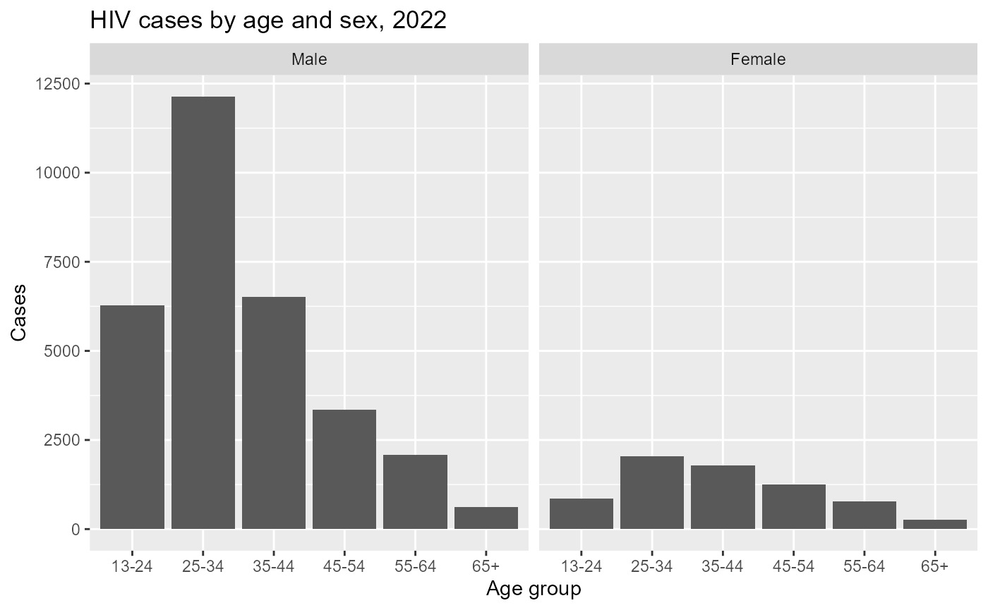
This allows direct comparison of age distributions by sex.
hiv_age_sex_summary <- hiv_age_sex %>%
  group_by(sex, age, indicator) %>%
  summarize(
    cases = sum(cases, na.rm = TRUE),
    .groups = "drop"
  )

hiv_age_sex_summary
#> # A tibble: 24 × 4
#>    sex   age   indicator       cases
#>    <fct> <fct> <fct>           <dbl>
#>  1 Male  13-24 HIV diagnoses    6273
#>  2 Male  13-24 HIV prevalence  22841
#>  3 Male  25-34 HIV diagnoses   12129
#>  4 Male  25-34 HIV prevalence 141323
#>  5 Male  35-44 HIV diagnoses    6524
#>  6 Male  35-44 HIV prevalence 164560
#>  7 Male  45-54 HIV diagnoses    3344
#>  8 Male  45-54 HIV prevalence 172264
#>  9 Male  55-64 HIV diagnoses    2089
#> 10 Male  55-64 HIV prevalence 226435
#> # ℹ 14 more rows
hiv_age_sex_summary%>%
  filter(indicator=="HIV diagnoses")%>%
  ggplot(aes(x = age, y = cases)) +
  geom_col() +
  facet_wrap(~ sex) +
  labs(
    title = "HIV cases by age and sex, 2022",
    x = "Age group",
    y = "Cases"
  )
Comparing years
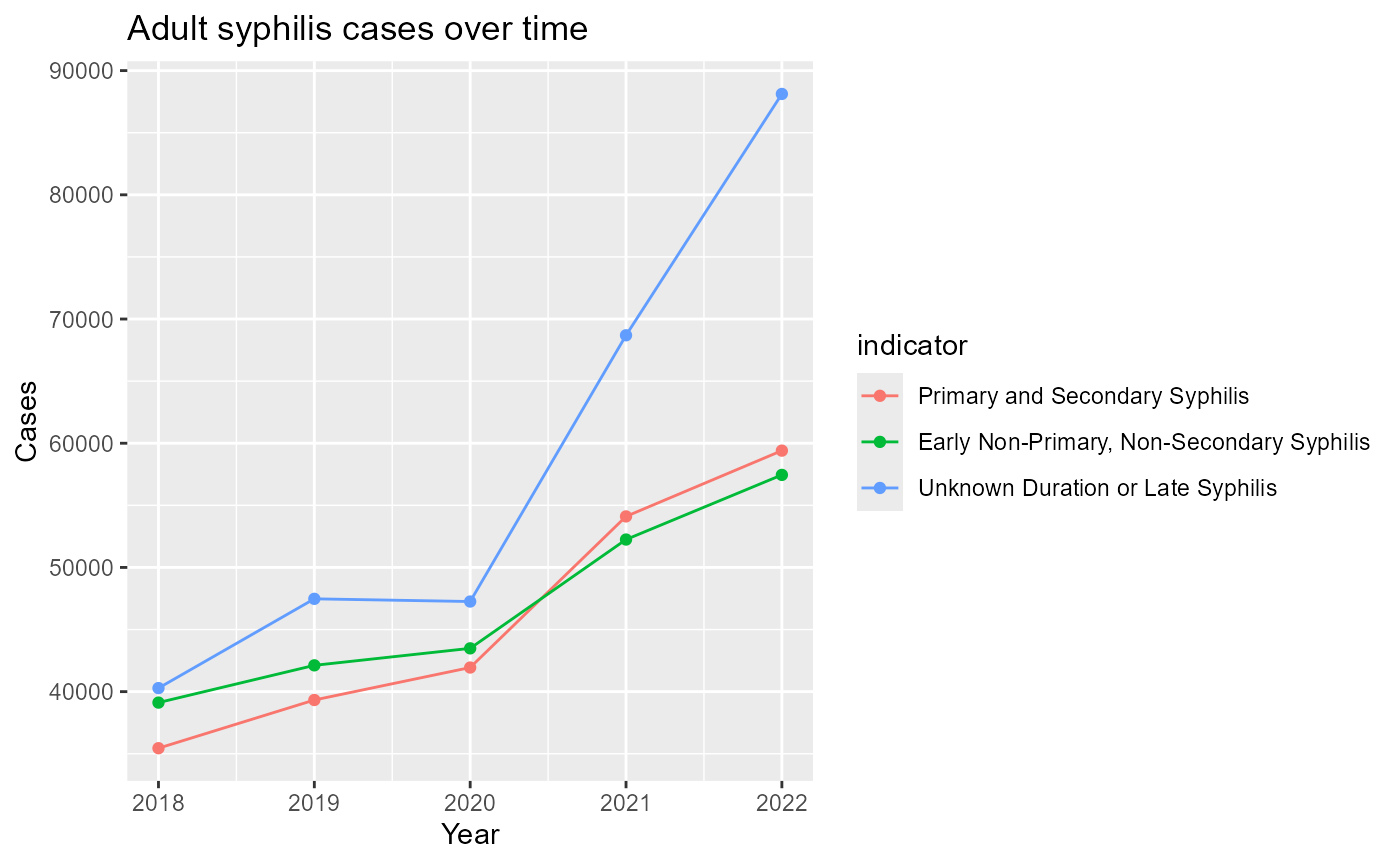
You can also query multiple years and compare trends over time.
syphilis_years <- get_atlas(
  disease   = "adult syphilis",
  geography = "state",
  year      = 2018:2022
)

head(syphilis_years)
#>                        indicator year geography    data_status
#> 1 Primary and Secondary Syphilis 2018   Alabama Not Suppressed
#> 2 Primary and Secondary Syphilis 2019   Alabama Not Suppressed
#> 3 Primary and Secondary Syphilis 2020   Alabama Not Suppressed
#> 4 Primary and Secondary Syphilis 2021   Alabama Not Suppressed
#> 5 Primary and Secondary Syphilis 2022   Alabama Not Suppressed
#> 6 Primary and Secondary Syphilis 2018    Alaska Not Suppressed
#>          race_ethnicity        sex            age                transmission
#> 1 All races/ethnicities Both sexes All age groups All transmission categories
#> 2 All races/ethnicities Both sexes All age groups All transmission categories
#> 3 All races/ethnicities Both sexes All age groups All transmission categories
#> 4 All races/ethnicities Both sexes All age groups All transmission categories
#> 5 All races/ethnicities Both sexes All age groups All transmission categories
#> 6 All races/ethnicities Both sexes All age groups All transmission categories
#>   rate100000 cases population lowerci_rate upperci_rate rse lowerci_cases
#> 1        9.8   477    4887681           NA           NA  NA            NA
#> 2       12.6   618    4903185           NA           NA  NA            NA
#> 3       10.5   529    5024279           NA           NA  NA            NA
#> 4       15.1   761    5039877           NA           NA  NA            NA
#> 5       23.5  1190    5074296           NA           NA  NA            NA
#> 6        7.5    55     735139           NA           NA  NA            NA
#>   upperci_cases fips
#> 1            NA   01
#> 2            NA   01
#> 3            NA   01
#> 4            NA   01
#> 5            NA   01
#> 6            NA   02
For example, compare national totals by year.
syphilis_trend <- syphilis_years %>%
  group_by(year, indicator) %>%
  summarize(
    cases = sum(cases, na.rm = TRUE),
    .groups = "drop"
  )

syphilis_trend
#> # A tibble: 15 × 3
#>     year indicator                                 cases
#>    <dbl> <fct>                                     <dbl>
#>  1  2018 Primary and Secondary Syphilis            35447
#>  2  2018 Early Non-Primary, Non-Secondary Syphilis 39119
#>  3  2018 Unknown Duration or Late Syphilis         40285
#>  4  2019 Primary and Secondary Syphilis            39327
#>  5  2019 Early Non-Primary, Non-Secondary Syphilis 42118
#>  6  2019 Unknown Duration or Late Syphilis         47473
#>  7  2020 Primary and Secondary Syphilis            41942
#>  8  2020 Early Non-Primary, Non-Secondary Syphilis 43486
#>  9  2020 Unknown Duration or Late Syphilis         47256
#> 10  2021 Primary and Secondary Syphilis            54108
#> 11  2021 Early Non-Primary, Non-Secondary Syphilis 52247
#> 12  2021 Unknown Duration or Late Syphilis         68691
#> 13  2022 Primary and Secondary Syphilis            59404
#> 14  2022 Early Non-Primary, Non-Secondary Syphilis 57450
#> 15  2022 Unknown Duration or Late Syphilis         88121
syphilis_trend%>%
ggplot(mapping= aes(x = year, y = cases, color=indicator, group=indicator)) +
  geom_line() +
  geom_point() +
  labs(
    title = "Adult syphilis cases over time",
    x = "Year",
    y = "Cases"
  )
Working with censored or missing values
CDC AtlasPlus may suppress or censor some values, especially for
small counts. Depending on the disease and geography, cases
or rate100000 may be missing.
A common first step is to inspect missingness.
Choosing diseases and stratification variables
The available diseases and stratification variables depend on CDC AtlasPlus. Common disease values include:
get_atlas(disease = "hiv", geography = "state", year = 2022)
get_atlas(disease = "chlamydia", geography = "state", year = 2022)
get_atlas(disease = "gonorrhea", geography = "state", year = 2022)
get_atlas(disease = "adult syphilis", geography = "state", year = 2022)
get_atlas(disease = "tuberculosis", geography = "state", year = 2022)
Next steps
After getting comfortable with basic queries, consider:
- querying multiple diseases
- comparing state and county results
- using sex, age, and race/ethnicity stratification
- joining AtlasPlus data to Census or spatial data
- using advanced vignettes for tract-level extrapolation and geographic access analyses
See ?get_atlas for full argument documentation.