UNOS Regions by State (sf), EPSG:5070 — UNOS_regions

Each row represents one U.S. state (contiguous U.S. plus the District of Columbia) annotated with its UNOS region. Geometries are state polygons projected to NAD83 / Conus Albers (EPSG:5070).

Usage

UNOS_regions_sf

Format

An sf object with one row per state and the following columns:

Region: UNOS region label (character)
State: State name as in the Census shapefile (character)
geometry: sfc_MULTIPOLYGON in EPSG:5070

Source

U.S. Census Bureau Cartographic Boundary Files (2018), states (20m).
UNOS region membership table from data-raw/UNOS regions.xlsx.

Details

The object is generated in data-raw/ by joining a table of UNOS region membership (state → region) to Census state boundaries and projecting once to a CONUS-appropriate projected CRS. Note this is state-level geometry; to obtain region polygons, dissolve by Region (see Examples).

Alaska, Hawaii, and Puerto Rico are excluded to focus on CONUS + DC, matching typical analytic maps and the chosen CRS. The original lat/long CRS of the shapefile is transformed to EPSG:5070 for consistent area/length behavior.

Examples

if (requireNamespace("sf", quietly = TRUE)) {
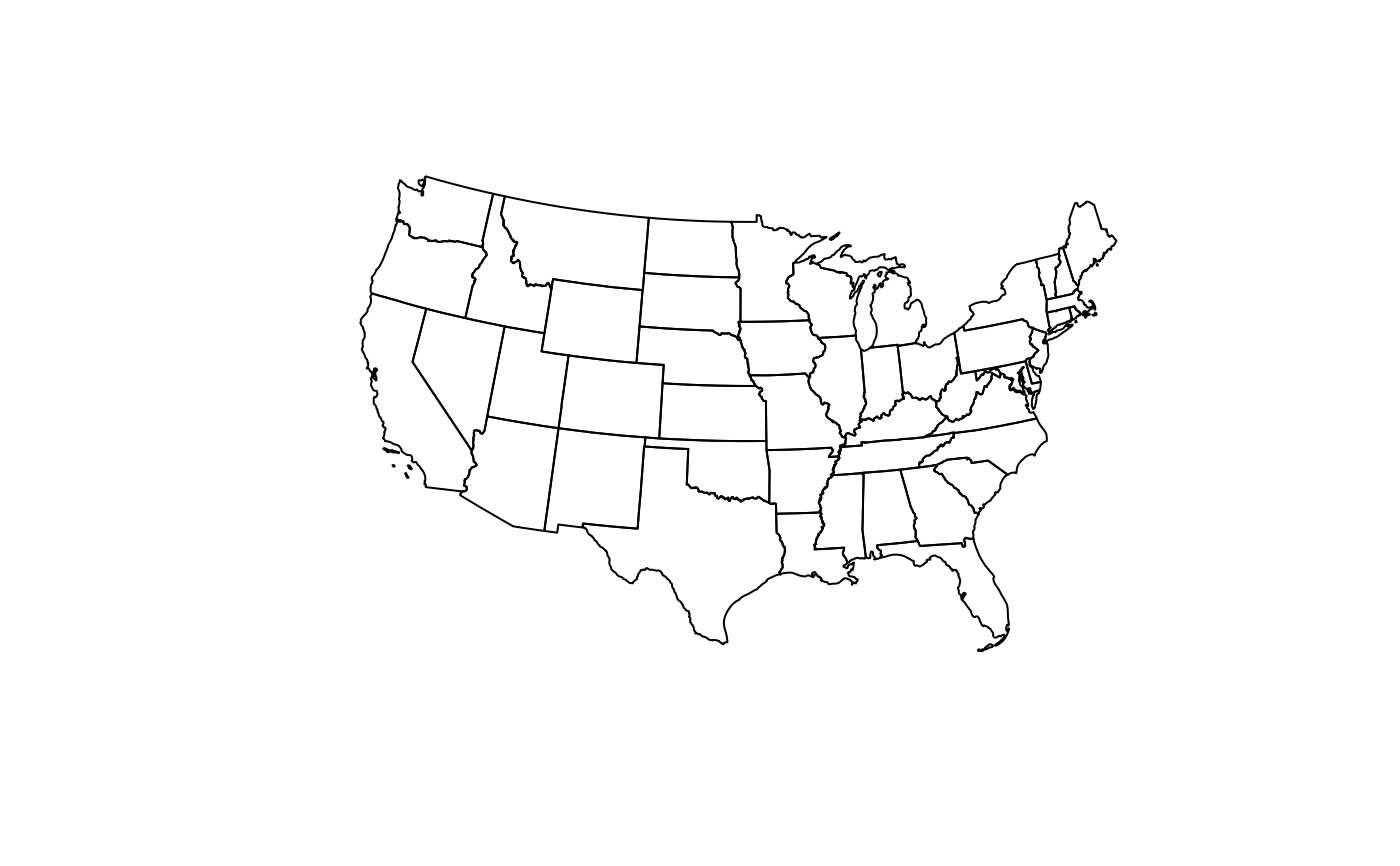
  # quick look
  plot(sf::st_geometry(UNOS_regions_sf))

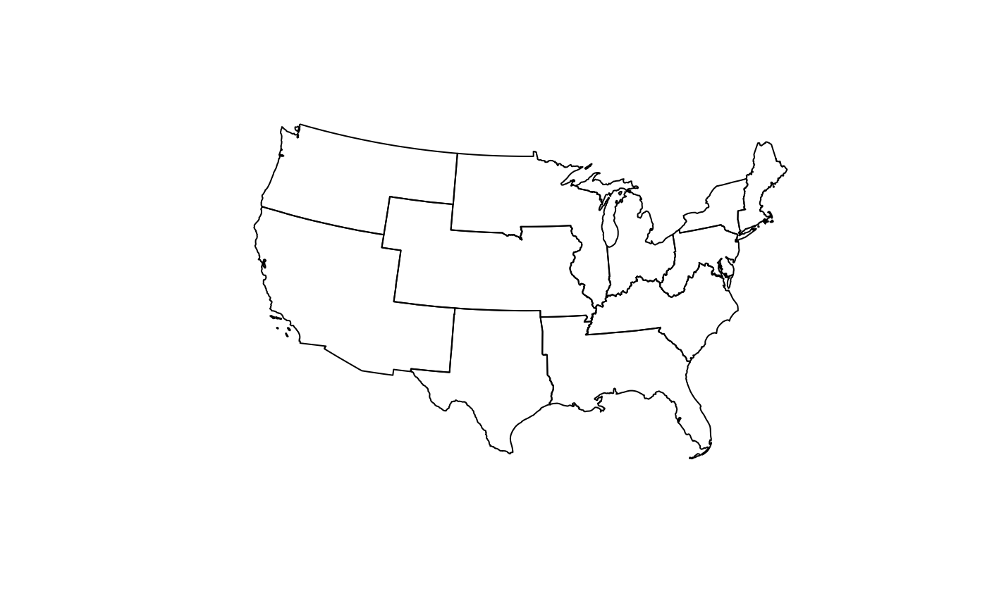
  # build dissolved region polygons if needed
  library(dplyr)
  unos_regions_poly <- UNOS_regions_sf %>%
    group_by(Region) %>%
    summarise(geometry = sf::st_union(geometry), .groups = "drop") %>%
    sf::st_make_valid()
  plot(sf::st_geometry(unos_regions_poly))
}

#> 
#> Attaching package: 'dplyr'
#> The following objects are masked from 'package:stats':
#> 
#>     filter, lag
#> The following objects are masked from 'package:base':
#> 
#>     intersect, setdiff, setequal, union